Differential Equations
Differential equations is without doubt one of the more useful branch of mathematics in science. They are used to model problems involving the change of some variable with respect to another. Differential equations cover a wide range of different applications, ranging from ordinary differential equations (ODE) until boundary-value problems involving many variables. For the sake of simplicity, throughout this section we shall cover only ODE systems as they are more elemental and equally useful. First, we shall cover first order methods, then second order methods and finally, system of differential equations.
import numpy as np
%pylab inline
import matplotlib.pyplot as plt
# JSAnimation import available at https://github.com/jakevdp/JSAnimation
from JSAnimation import IPython_display
from matplotlib import animation
Populating the interactive namespace from numpy and matplotlib
First Order Methods
Ordinary differential equations normally implies the solution of an initial-value problem, i.e., the solution has to satisfy the differential equation together with some initial condition. Real-life problems usually imply very complicated problems and even non-soluble ones, making any analytical approximation unfeasible. Fortunately, there are two ways to handle this. First, for almost every situation, it is generally posible to simplify the original problem and obtain a simpler one that can be easily solved. Then, using perturbation theory, we can perturbate this solution in order to approximate the real one. This approach is useful, however, it depends very much on the specific problem and a systematic study is rather complicated.
The second approximation, and the one used here, consists of a complete numerical reduction of the problem, solving it exactly within the accuracy allowed by implicit errors of the methods. For this part, we are going to assume well-defined problems, where solutions are expected to be well-behaved.
Euler's method
This method is the most basic of all methods, however, it is useful to understand basic concepts and definitions of differential equations problems.
Suppose we have a well-posed initial-value problem given by:
$$ \frac{dy}{dt}=f(t,y),\ \ \ a\leq t\leq b, \ \ \ \ y(a) = \alpha $$Now, let's define a mesh points as a set of values $\{t_i\}t_i$ where we are going to approximate the solution $y(t)$. These points can be equal-spaced such that
$$ t_i = a+ i h,\ \ \ \ \mbox{with}\ \ i=1,2,3,\cdots,N \ \ \mbox{and}\ h = \frac{b-a}{N}. $$Here, $h$ is called the step size of the mesh points.
Now, using the first-order approximation of the derivative saw in Numerical Differentiation, we obtain
$$ \frac{dy}{dt}\approx \frac{y(t+h)-y(t)}{h} $$or
$$ \left.\frac{dy}{dt}\right|_{t=t_i}\approx \frac{y(t_{i+1})-y(t_i)}{h} $$The original problem can be rewritten as
$$ y_{i+1} = y_i + hf(t_i, y_i) + \frac{h^2}{2}y^{''}(\xi_i) $$where the notation $y(t_i)\equiv y_i$ has been introduced and the last term (error term) can be obtained taking a second-order approximation of the derivative.
This equation can be solved recursively as we know the initial value $y_0 = y(a) = \alpha$.
Example 1
The formalism of the Euler's method can be applied for any system of the form:
$$ \frac{dy}{dt}=f(t,y),\ \ \ a\leq t\leq b, \ \ \ \ y(a) = \alpha $$However, it is possible to extend this to second-order systems, i.e., systems involving second derivatives. Let's suppose a general system of the form:
$$ \frac{d^2y}{dt^2}+ g(t,y)\frac{dy}{dt}=f(t,y),\ \ \ a\leq t\leq b, \ \ \ \ y(a) = \alpha\ \ \mbox{and}\ y'(a) = \beta$$For this system we have to provide both, the initial value $y(a)$ and the initial derivative $y'(a)$.
Now, let's define a new variable $w(t) = y'(t)$, the previous problem can be then written as
$$ \matrix{\frac{dw}{dt}=g(t,y)w-f(t,y) \\ \frac{dy}{dt}=w(t)} ,\ \ \ a\leq t\leq b, \ \ \ \ y(a) = \alpha\ \ \mbox{and}\ w(a) = \beta$$Each of this problem has now the form required by the Euler's algorithm, and the solution can be computed as:
$$ \matrix{w_{i+1}= w_{i} + h[g(t_i,y_i)w_i-f(t_i,y_i)] \\ y_{i+1}=y_i + hw_i} ,\ \ \ a\leq t\leq b, \ \ \ \ y(a) = \alpha\ \ \mbox{and}\ w(a) = \beta$$In order to apply this, let's assume a simple mass-spring.
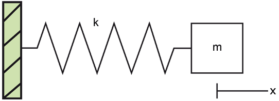
The equation of motion according to Newton's second law is
$$ m\frac{d^2x}{dt^2} = -kx $$Using the previous results, we can rewrite this as:
$$ \frac{dv}{dt} = -\frac{k}{m}x $$$$ \frac{dx}{dt} = v $$And the equivalent Euler system is
$$ \matrix{v_{i+1}= v_{i} - h\frac{k}{m}x_i \\ x_{i+1}=x_i + hv_i} ,\ \ \ x(0) = x_0\ \ \mbox{and}\ v(0) = v_0$$Activity 
High Order Methods
Although first-order schemes like Euler's method are illustrative and allow a good understanding of the numerical problem, real applications cannot be dealt with them, instead more precise and accurate high-order methods must be invoked. In this section we shall cover a well-known family of numerical integrators, the Runge-Kutta methods.
Second-order Runge-Kutta methods
For this method, let's assume a problem of the form:
$$ \frac{dy}{dt}=y'=f(t,y),\ \ \ a\leq t\leq b, \ \ \ \ y(a) = \alpha $$Now, we want to know the solution in the next timestep, i.e. $y(t+h)$. For this, we propose the next solution:
$$ y(t+h) = y(t) + c_0 f(t,y)h + c_1f[ t+ph, y+qhf(t,y) ]h $$determining the coefficients $c_0, c_1, q$ and $p$, we will have the complete approximated solution of the problem.
One way to determine them is by comparing with the taylor expansion around $t$
$$ y(t+h) = y(t) + f(t,y)h + \frac{1}{2}\left( \frac{\partial f}{\partial t} + \frac{\partial f}{\partial y} \right)h^2 + \mathcal{O}(h^3) $$Now, we can also expand the function $f[ t+ph, y+qhf(t,y) ]$ around the point $(t,y)$, yielding:
$$ f[ t+ph, y+qhf(t,y) ] = f(t,y) + \frac{\partial f}{\partial t}ph + \frac{\partial f}{\partial y}qh + \mathcal{O}(h^2) $$Replacing this into the original expression:
$$ y(t+h) = y(t) + c_0 f(t,y)h + c_1\left[ f(t,y) + \frac{\partial f}{\partial t}ph + \frac{\partial f}{\partial y}qh \right]h + \mathcal{O}(h^3)$$ordering the terms we obtain:
$$ y(t+h) = y(t) + (c_0+c_1) f(t,y)h + c_1\left[ \frac{\partial f}{\partial t}p + \frac{\partial f}{\partial y}q \right]h^2 + \mathcal{O}(h^3)$$Equalling the next conditions are obtained:
$$ c_0 + c_1 =1 \ \ \ c_1p=\frac{1}{2}\ \ \ c_1q = \frac{1}{2} $$This set of equations are undetermined so there are several solutions, each one yielding a different method:
$$ \matrix{ c_0 = 0 & c_1=1 & p = 1/2 & q = 1/2 & \mbox{Modified Euler's Method} \\ c_0 = 1/2 & c_1=1/2 & p = 1 & q = 1 & \mbox{Heun's Method} \\ c_0 = 1/3 & c_1=2/3 & p = 3/4 & q = 3/4 & \mbox{Ralston's Method} } $$The algorithm is then:
$$ y(t+h) = y(t) + (c_1+c_2)\mathbf{K}_1 $$with
$$ \mathbf{K}_1 = hf( t+pt, y+q\mathbf{K}_0 ) $$$$ \mathbf{K}_0 = hf(t,y) $$All these methods constitute the second-order Runge-Kutta methods.
Example 2
In this example we are going to use the Runge-Kutta 2 method (Modified Euler's) for mapping the phase space of a pendulum.
The equations of the pendulum are given by:
$$ \theta' = \omega $$$$ \omega' = -\frac{g}{l}\sin(\theta) $$#RK2 integrator
def RK2_step( f, y, t, h ):
#Creating solutions
K0 = h*f(t, y)
K1 = h*f(t + 0.5*h, y + 0.5*K0)
y1 = y + K1
#Returning solution
return y1
The phase space of a dynamical system is a space in which all the possible states of that system are univocally represented. For the case of the pendulum, a complete state of the system is given by the set $(\theta, \omega)$, so its phase space is two-dimensional. In order to explore all the possible states, we are going to generate a set of initial conditions and integrate them.
#========================================================
#Defining parameters
#========================================================
#Gravity
g = 9.8
#Pendulum's lenght
l = 1.0

#Number of initial conditions
Nic = 1000
#Maxim angular velocity
omega_max = 8

#Maxim time of integration
tmax = 6*np.pi
#Timestep
h = 0.01

#========================================================
#Dynamical function of the system
#========================================================
def function( t, y ):
    #Using the convention y = [theta, omega]
    theta = y[0]
    omega = y[1]
    #Derivatives
    dtheta = omega
    domega = -g/l*np.sin(theta)
    return np.array([dtheta, domega])
#========================================================
#Generating set of initial conditions
#========================================================
theta0s = -4*np.pi + np.random.random(Nic)*8*np.pi
omega0s = -omega_max + np.random.random(Nic)*2*omega_max


#========================================================
#Integrating and plotting the solution for each IC
#========================================================
#Setting figure
plt.figure( figsize = (8,5) )
for theta0, omega0 in zip(theta0s, omega0s):
    #Arrays for solutions
    time = [0,]
    theta = [theta0,]
    omega = [omega0,]
    for i, t in zip(xrange(int(tmax/h)), np.arange( 0, tmax, h )):
        #Building current condition
        y = [theta[i], omega[i]]
        #Integrating the system
        thetai, omegai = RK2_step( function, y, t, h )
        #Appending new components
        theta.append( thetai )
        omega.append( omegai )
        time.append( t )
    #Plotting solution
    plt.plot( theta, omega, lw = 0.1, color = "black" )

#Format of figure
plt.xlabel( "$\\theta$", fontsize = 18 )
plt.ylabel( "$\omega$", fontsize = 18 )
plt.xlim( (-2*np.pi, 2*np.pi) )
plt.ylim( (-omega_max, omega_max) )
plt.title( "Phase space of a pendulum" )
plt.grid(1)

Activity 
Fourth-order Runge-Kutta method
Finally, the most used general purpose method is the fourth-order Runge-Kutta scheme. Its derivation follows the same previous reasoning, however the procedure is rather long and it makes no sense to reprouce it here. Instead, we will give the direct algorithm:
Let's assume again a problem of the form:
$$ \frac{dy}{dt}=y'=f(t,y),\ \ \ a\leq t\leq b, \ \ \ \ y(a) = \alpha $$The Runge-Kutta-4 (RK4) method allows us to predict the solution at the time $t+h$ as:
$$ y(t+h) = y(t) + \frac{1}{6}( \mathbf{K}_0 + 2\mathbf{K}_1 + 2\mathbf{K}_2 + \mathbf{K}_3 ) $$where:
$$ \mathbf{K}_0 = hf(t,y)$$$$ \mathbf{K}_1 = hf\left( t + \frac{h}{2},y + \frac{\mathbf{K}_0}{2}\right)$$$$ \mathbf{K}_2 = hf\left( t + \frac{h}{2},y + \frac{\mathbf{K}_1}{2}\right)$$$$ \mathbf{K}_3 = hf\left( t + h,y + \mathbf{K}_2\right)$$Activity 
with $a = 10$, $b=28$ and $c = 8/3$ the solution shows periodic orbits.
Two-Point Boundary Value Problems
Up to now we have solved initial value problems of the form:
$$ \frac{dy}{dt}=y'=f(t,y),\ \ \ a\leq t\leq b, \ \ \ \ y(a) = \alpha $$Second order equations can be similarly planted as
$$ \frac{d^2y}{dt^2}=y''=f(t,y,y'),\ \ \ a\leq t\leq b, \ \ \ \ y(a) = \alpha \ \ \ y'(a) = u $$This type of systems can be readily solved by defining the auxiliar variable $w = y'$, turning it into a first order system of equations.
Now, we shall solve two-point boundary problem, where we have two conditions on the solution $y(t)$ instead of having the function and its derivative at some initial point, i.e.
$$ \frac{d^2y}{dt^2}=y''=f(t,y,y'),\ \ \ a\leq t\leq b, \ \ \ \ y(a) = \alpha \ \ \ y(b) = \beta $$In spite of its similar form to the initial value problem, two-point boundary problems pose a increased difficulty for numerical methods. The main reason of this is the iterative procedure performed by numerical approaches, where from an initial point, further points are found. Trying to fit two different values at different points implies then a continuous readjusting of the solution.
A common way to solve these problems is by turning them into a initial-value problem
$$ \frac{d^2y}{dt^2}=y''=f(t,y,y'),\ \ \ a\leq t\leq b, \ \ \ \ y(a) = \alpha \ \ \ y'(a) = u $$Let's suppose some choice of $u$, integrating by using some of the previous methods, we obtain the final boundary condition $y(b)=\theta$. If the produced value is not the one we wanted from our initial problem, we try another value $u$. This can be repeated until we get a reasonable approach to $y(b)=\beta$. This method works fine, but it is so expensive and terribly inefficient.
Note when we change $u$, the final boundary value also change, so we can assume $y(b) = \theta$. The solution to the problem can be thought then as a root-finding problem:
$$ y(b) = \theta(u) = \beta $$or
$ r(u) \equiv \theta(u) - \beta = 0 $
where $r(u)$ is the residual function. This problem can be thus solved using some of the methods previously seen for the root-finding problem.
Example 3
A very simplified model of interior solid planets consists of a set of spherically symmetric radial layers, where the next properties are computed: density $\rho(r)$, enclosed mass $m(r)$, gravity $g(r)$ and pressure $P(r)$. Each of these properties are assumed to be only radially dependent. The set of equations that rules the planetary interior is:
Hydrostatic equilibrium equation
$$\frac{dP}{dr} = -\rho(r)g(r)$$Adams-Williamson equation
$$\frac{dg}{dr} = 4\pi G\rho(r) - \frac{2Gm(r)}{r^3}$$Continuity equation
$$\frac{dm}{dr} = 4\pi r^2 \rho(r)$$Equation of state
$$\frac{d\rho}{dr} = -\frac{\rho(r)^2g(r)}{K_s}$$For accurate results the term $K_s$, called the adiabatic bulk modulus, is temperature and radii dependent. However, for the sake of simplicity we shall assume a constant value.
Solving simultaneously the previous set of equations, we can find the complete internal structure of a planet.
We have four functions to be determined and four equations, so the problem is solvable. It is only necessary to provide a set of boundary conditions of the form:
$$ \rho(R) = \rho_{surf},\ \ \ m(R) = M_p, \ \ \ g(R) = g_{surf},\ \ \ P(R) = P_{atm} $$where $R$ is the planetary radius, $\rho_{surf}$ the surface density, $M_p$ the mass of the planet, $g_{surf}$ the surface gravity and $P_{atm}$ the atmospheric pressure. However, there is a problem, we do not know the planetary radius $R$, so an extra condition is required to determine this value. This is reached through the physical condition $m(0) = 0$, this is, the enclosed mass at a radius $r = 0$ (center of the planet) must be 0.
The two-value boundary nature of this problem lies then in fitting the mass function at $m(R) = M_p$ and at $m(0) = 0$. To do so, let's call the residual mass $m(0) = M_r$. This value should depend on the chosen radius $R$, so a large value would imply a mass defect $M_r(R)<0$, and a small value a mass excess $M_r(0)>0$. The problem is then solving the radius $R$ for which $m(0) = M_r(R) = 0$. This can be done by using the bisection method.
For this problem, we are going to assume an one-layer planet made of perovskite, so $K_s \approx 200\ GPa$. A planet mass equal to earth, so $M_p = 5.97219 \times 10^{24}\ kg$, a surface density $\rho_{surf} = 3500\ kg/m^3$ and a atmospheric pressure of $P_{atm} = 1\ atm = 1\times 10^5\ Pa$.