Numerical Calculus
Throughout this section and the next ones, we shall cover the topic of numerical calculus. Calculus has been identified since ancient times as a powerful toolkit for analysing and handling geometrical problems. Since differential calculus was developed by Newton and Leibniz (in its actual notation), many different applications have been found, at the point that most of the current science is founded on it (e.g. differential and integral equations). Due to the ever increasing complexity of analytical expressions used in physics and astronomy, their usage becomes more and more impractical, and numerical approaches are more than necessary when one wants to go deeper. This issue has been identified since long ago and many numerical techniques have been developed. We shall cover only the most basic schemes, but also providing a basis for more formal approaches.
import numpy as np
%pylab inline
import matplotlib.pyplot as plt
# JSAnimation import available at https://github.com/jakevdp/JSAnimation
from JSAnimation import IPython_display
from matplotlib import animation
#Interpolation add-on
import scipy.interpolate as interp
Populating the interactive namespace from numpy and matplotlib
WARNING: pylab import has clobbered these variables: ['interp']
`%pylab --no-import-all` prevents importing * from pylab and numpy
Numerical Differentiation
According to the formal definition of differentiation, given a function $f(x)$ such that $f(x)\in C^1[a,b]$, the first order derivative is given by
$$\frac{d}{dx}f(x) = f'(x) = \lim_{h\rightarrow 0} \frac{f(x+h)-f(x)}{h}$$However, when $f(x)$ exhibits a complex form or is a numerical function (only a discrete set of points are known), this expression becomes unfeasible. In spite of this, this formula gives us a very first rough way to calculate numerical derivatives by taking a finite interval $h$, i.e.
$$f'(x) \approx \frac{f(x+h)-f(x)}{h}$$where the function must be known at least in $x_0$ and $x_1 = x_0+h$, and $h$ should be small enough.
Example 1
Evaluate the first derivative of the next function using the previous numerical scheme at the point $x_0=2.0$ and using $h=0.5,\ 0.1,\ 0.05$
$f(x) = \sqrt{1+\cos^2(x)}$
Compare with the real function and plot the tangent line using the found values of the slope.
#Function to evaluate
def function(x):
    return np.sqrt( 1+np.cos(x)**2 )

#X value
x0 = 2
xmin = 1.8
xmax = 2.2
#h step
hs = [0.5,0.1,0.05]

#Calculating derivatives
dfs = []
for h in hs:
    dfs.append( (function(x0+h)-function(x0))/h )

#Plotting
plt.figure( figsize=(10,8) )
#X array
X = np.linspace( xmin, xmax, 100 )
Y = function(X)
plt.plot( X, Y, color="black", label="function", linewidth=3, zorder=10 )
#Slopes
Xslp = [1,x0,3]
Yslp = [0,0,0]
for df, h in zip(dfs, hs):
    #First point
    Yslp[0] = function(x0)+df*(Xslp[0]-Xslp[1])
    #Second point
    Yslp[1] = function(x0)
    #Third point
    Yslp[2] = function(x0)+df*(Xslp[2]-Xslp[1])
    #Plotting this slope
    plt.plot( Xslp, Yslp, linewidth = 2, label="slope$=%1.2f$ for $h=%1.2f$"%(df,h) )

#Format
plt.grid()
plt.xlabel("x")
plt.ylabel("y")
plt.xlim( xmin, xmax )
plt.ylim( 1, 1.15 )
plt.legend( loc = "upper left" )
<matplotlib.legend.Legend at 0x7f2790fe7990>

n+1-point formula
A generalization of the previous formula is given by the (n+1)-point formula, where first-order derivatives are calculated using more than one point, what makes it a much better approximation for many problems.
Theorem
For a function $f(x)$ such that $f(x)\in C^{n+1}[a,b]$, the next expression is always satisfied
$$f(x) = P(x) + \frac{f^{(n+1)}(\xi(x))}{(n+1)!}(x-x_0)(x-x_1)\cdots(x-x_n)$$where $\{x_i\}_i$ is a set of point where the function is mapped, $\xi(x)$ is some function of $x$ such that $\xi\in[a,b]$, and $P(x)$ is the associated Lagrange interpolant polynomial.
As $n$ becomes higher, the approximation should be better as the error term becomes neglectable.
Taking the previous expression, and differenciating, we obtain
$$f(x) = \sum_{k=0}^n f(x_k)L_{n,k}(x) + \frac{(x-x_0)(x-x_1)\cdots(x-x_n)}{(n+1)!}f^{(n+1)}(\xi(x))$$$$f'(x_j) = \sum_{k=0}^n f(x_k)L'_{n,k}(x_j) + \frac{f^{(n+1)}(\xi(x_j))}{(n+1)!} \prod_{k=0,k\neq j}^{n}(x_j-x_k)$$where $L_{n,k}$ is the $k$-th Lagrange basis functions for $n$ points, $L'_{n,k}$ is its first derivative.
Note that the last expressions is evaluated in $x_j$ rather than a general $x$ value, the cause of this is because this expression is not longer valid for another value not within the set $\{x_i\}_i$, however this is not an inconvenient when handling real applications.
This formula constitutes the (n+1)-point approximation and it comprises a generalization of almost all the existing schemes to differentiate numerically. Next, we shall derive some very used formulas.
For example, the form that takes this derivative polynomial for 3 points $(x_i,y_i)$ is the following
$$f'(x_j) = f(x_0)\left[ \frac{2x_j-x_1-x_2}{(x_0-x_1)(x_0-x_2)}\right] + f(x_1)\left[ \frac{2x_j-x_0-x_2}{(x_1-x_0)(x_1-x_2)}\right] + f(x_2)\left[ \frac{2x_j-x_0-x_1}{(x_2-x_0)(x_2-x_1)}\right] $$$$\hspace{2cm} + \frac{1}{6} f^{(3)}(\epsilon_j) \prod_{k=0,k\neq j}^{n}(x_j-x_k)$$
Endpoint formulas
Endpoint formulas are based on evaluating the derivative at the first of a set of points, i.e., if we want to evaluate $f'(x)$ at $x_i$, we then need $(x_i$, $x_{i+1}=x_i+h$, $x_{i+2}=x_i+2h$, $\cdots)$. For the sake of simplicity, it is usually assumed that the set $\{x_i\}_i$ is equally spaced such that $x_k = x_0+k\cdot h$.
Three-point Endpoint Formula
$$f'(x_i) = \frac{1}{2h}[-3f(x_i)+4f(x_i+h)-f(x_i+2h)] + \frac{h^2}{3}f^{(3)}(\xi)$$with $\xi\in[x_i,x_i+2h]$
Five-point Endpoint Formula
$$f'(x_i) = \frac{1}{12h}[-25f(x_i)+48f(x_i+h)-36f(x_i+2h)+16f(x_i+3h)-3f(x_i+4h)] + \frac{h^4}{5}f^{(5)}(\xi)$$with $\xi\in[x_i,x_i+4h]$
Endpoint formulas are especially useful near to the end of a set of points, where no further points exist.
Midpoint formulas
On the other hand, Midpoint formulas are based on evaluating the derivative at the middle of a set of points, i.e., if we want to evaluate $f'(x)$ at $x_i$, we then need $(\cdots$, $x_{i-2} = x_i - 2h$, $x_{i-1} = x_i - h$, $x_i$, $x_{i+1}=x_i+h$, $x_{i+2}=x_i+2h$, $\cdots)$.
Three-point Midpoint Formula
$$f'(x_i) = \frac{1}{2h}[f(x_i+h)-f(x_i-h)] + \frac{h^2}{6}f^{(3)}(\xi)$$with $\xi\in[x_i-h,x_i+h]$
Five-point Midpoint Formula
$$f'(x_i) = \frac{1}{12h}[f(x_i-2h)-8f(x_i-h)+8f(x_i+h)-f(x_i+2h)] + \frac{h^4}{30}f^{(5)}(\xi)$$with $\xi\in[x_i-2h,x_i+2h]$
As Midpoint formulas required one iteration less than Endpoint ones, they are more often used for numerical applications. Furthermore, the round-off error is smaller as well. However, near to the end of a set of points, they are no longer useful as no further points exists, and Endpoint formulas are preferable.
#Derivative three end point

def TEP( Yn,i, h=0.01,right=0 ):
    suma = -3*Yn[i]+4*Yn[i+(-1)**right*1]-Yn[i+(-1)**right*2]
    return suma/(2*h*(-1)**right)

#Derivative mid point
def TMP( Ynh,Ynmh, h = 0.01 ):
    return (Ynh-Ynmh)/(2*h)
Example: Heat transfer in a 1D bar
Fourier's Law of thermal conduction describes the diffusion of heat. Situations in which there are gradients of heat, a flux that tends to homogenise the temperature arises as a consequence of collisions of particles within a body. The Fourier's Law is giving by
$$ q = -k\nabla T = -k\left( \frac{dT}{dx}\hat{i} + \frac{dT}{dy}\hat{j} + \frac{dT}{dz}\hat{k}\right)$$where T is the temperature, $\nabla T$ its gradient and k is the material's conductivity. In the next example it is shown the magnitud of the heat flux in a 1D bar(wire).
#Temperature profile
def Temp(x):
    return x**3 + 3*x-1

# Points where function is known
Xn = np.linspace(0,10,100)
Tn = Temp(Xn)
#Magnitude of heat flux array
Q = np.zeros(len(Xn))
#Left end derivative
Q[0] = TEP(Tn,0)

#Mid point derivatives
index = len(Xn)-1
for i in xrange( 1,index ):
    Q[i] =  TMP( Tn[i+1],Tn[i-1] )

#Right end derivative
Q[-1] = TEP( Tn,index,right=1 )

#Plotting
plt.figure( figsize=(8,7) )
plt.plot(Xn,Q)

plt.grid()
plt.xlabel( "x",fontsize =15 )
plt.ylabel( "$\\frac{dT}{dx}$",fontsize =20 )
plt.title( " Magnitud heat flux transfer in 1D bar" )
<matplotlib.text.Text at 0x7f2790ddd4d0>

Activity 
Construct a density map of the magnitud of the heat flux of a 2D bar. Consider the temperature profile as $$ T(x,y) = x^3 + 3x-1+y^2 $$
Activity 
Activity 
The radar stations A and B, separated by the distance a = 500 m, track the plane C by recording the angles $\alpha$ and $\beta$ at 1-second intervals. The successive readings are
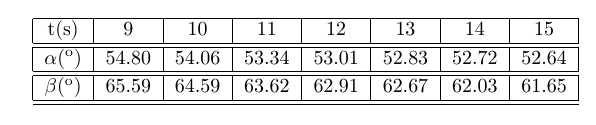
calculate the speed v using the 3 point approximantion at t = 10 ,12 and 14 s. Calculate the x component of the acceleration of the plane at = 12 s. The coordinates of the plane can be shown to be
\begin{equation} x = a\frac{\tan \beta}{\tan \beta- \tan \alpha}\\ y = a\frac{\tan \alpha\tan \beta}{\tan \beta- \tan \alpha} \end{equation}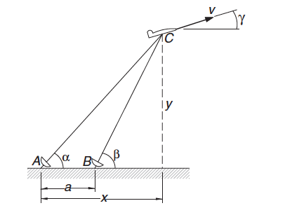
Numerical Integration
Integration is the second fundamental concept of calculus (along with differentiation). Numerical approaches are generally more useful here than in differentiation as the antiderivative procedure (analytically) is often much more complex, or even not possible. In this section we will cover some basic schemes, including numerical quadratures.
Geometrically, integration can be understood as the area below a funtion within a given interval. Formally, given a function $f(x)$ such that $f\in C^{1}[a,b]$, the antiderivative is defined as
$$F(x) = \int f(x) dx$$valid for all $x$ in $[a,b]$. However, a more useful expression is a definite integral, where the antiderivative is evaluated within some interval, i.e.
$$F(x_1) - F(x_0) = \int_{x_0}^{x_1} f(x) dx$$This procedure can be formally thought as a generalization of discrete weighted summation. This idea will be exploited below and will lead us to some first approximations to integration.
Numerical quadrature
Given a well-behaved function $f(x)$, a previous theorem guarantees that
$$f(x) = \sum_{k=0}^n f(x_k)L_{n,k}(x) + \frac{(x-x_0)(x-x_1)\cdots(x-x_n)}{(n+1)!}f^{(n+1)}(\xi(x))$$with $L_{n,k}(x)$ the lagrange basis functions. Integrating $f(x)$ over $[a,b]$, we obtain the next expression:
$$\int_a^b f(x)dx = \int_a^b\sum_{k=0}^n f(x_k)L_{n,k}(x)dx + \int_a^b\frac{(x-x_0)(x-x_1)\cdots(x-x_n)}{(n+1)!}f^{(n+1)}(\xi(x))dx$$It is worth mentioning this expression is a number, unlike differentiation where we obtained a function.
We can readily convert this expression in a weighted summation as
$$\int_a^b f(x)dx = \sum_{k=0}^n a_if(x_k) + \frac{1}{(n+1)!}\int_a^bf^{(n+1)}(\xi(x)) \prod_{k=0}^{n}(x-x_k)dx$$where each coefficient is defined as:
$$a_i = \int_a^b L_{n,k}(x) dx = \int_a^b\prod_{j=0,\ j\neq k}^{n}\frac{(x-x_j)}{(x_k-x_j)}dx$$Finally, the quadrature formula or Newton-Cotes formula is given by the next expression:
$$\int_a^b f(x) dx = \sum a_i f(x_i) + E[f]$$where the estimated error is
$$E[f] = \frac{1}{(n+1)!}\int_a^bf^{(n+1)}(\xi(x)) \prod_{k=0}^{n}(x-x_k)dx $$Asumming besides intervals equally spaced such that $x_i = x_0 + i\times h$, the error formula becomes:
$$E[f] = \frac{h^{n+3}f^{n+2}(\xi)}{(n+1)!}\int_0^nt^2(t-1)\cdots(t-n) $$if $n$ is even and
$$E[f] = \frac{h^{n+2}f^{n+1}(\xi)}{(n+1)!}\int_0^nt(t-1)\cdots(t-n) $$if $n$ is odd.
#Quadrature method
def Quadrature( f, X, xmin, xmax, ymin=0, ymax=1, fig=None, leg=True ):
    #f(x_i) values
    Y = f( X )

    #X array
    Xarray = np.linspace( xmin, xmax, 1000 )
    #X area
    Xarea = np.linspace( X[0], X[-1], 1000 )
    #F array
    Yarray = f( Xarray )

    #Lagrange polynomial
    Ln = interp.lagrange( X, Y )
    #Interpolated array
    Parray = Ln( Xarray )
    #Interpolated array for area
    Parea = Ln( Xarea )

    #Plotting
    if fig==None:
        fig = plt.figure( figsize = (8,8) )
    ax = fig.add_subplot(111)
    #Function
    ax.plot( Xarray, Yarray, linewidth = 3, color = "blue", label="$f(x)$" )
    #Points
    ax.plot( X, Y, "o", color="red", label="points", zorder = 10 )
    #Interpolator
    ax.plot( Xarray, Parray, linewidth = 2, color = "black", label="$P_{%d}(x)$"%(len(X)-1) )
    #Area
    ax.fill_between( Xarea, Parea, color="green", alpha=0.5 )

    #Format
    ax.set_title( "%d-point Quadrature"%(len(X)), fontsize=16 )
    ax.set_xlim( (xmin, xmax) )
    ax.set_ylim( (0, 4) )
    ax.set_xlabel( "$x$" )
    ax.set_ylabel( "$y$" )
    if leg:
        ax.legend( loc="upper left", fontsize=16 )
    ax.grid(1)

    return ax
Trapezoidal rule
Using the previous formula, it is easily to derivate a set of low-order approximations for integration. Asumming a function $f(x)$ and an interval $[x_0,x_1]$, the associated quadrature formula is that obtained from a first-order Lagrange polynomial $P_1(x)$ given by:
$$P_1(x) = \frac{(x-x_1)}{x_0-x_1}f(x_0) + \frac{(x-x_0)}{(x_1-x_0)}f(x_1)$$Using this, it is readible to obtain the integrate:
$$\int_{x_0}^{x_1}f(x)dx = \frac{h}{2}[ f(x_0) + f(x_1) ]-\frac{h^3}{12}f^{''}(\xi)$$with $\xi \in [x_0, x_1]$ and $h = x_1-x_0$.
#Function
def f(x):
    return 1+np.cos(x)**2+x

#Quadrature with 2 points (Trapezoidal rule)
X = np.array([-0.5,1.5])
Quadrature( f, X, xmin=-1, xmax=2, ymin=0, ymax=4 )
<matplotlib.axes.AxesSubplot at 0x7f7dfa4b3f50>

Simpson's rule
A slightly better approximation to integration is the Simpson's rule. For this, assume a function $f(x)$ and an interval $[x_0,x_2]$, with a intermediate point $x_1$. The associate second-order Lagrange polynomial is given by:
$$P_2(x) = \frac{(x-x_1)(x-x_2)}{(x_0-x_1)(x_0-x_2)}f(x_0) + \frac{(x-x_0)(x-x_2)}{(x_1-x_0)(x_1-x_2)}f(x_1) + \frac{(x-x_0)(x-x_1)}{(x_2-x_0)(x_2-x_1)}f(x_2)$$The final expression is then:
$$\int_{x_0}^{x_2} f(x)dx = \frac{h}{3}[ f(x_0)+4f(x_1)+f(x_2) ]-\frac{h^5}{90}f^{(4)}(\xi)$$#Function
def f(x):
return 1+np.cos(x)**2+x
#Quadrature with 3 points (Simpson's rule)
X = np.array([-0.5,0.5,1.5])
Quadrature( f, X, xmin=-1, xmax=2, ymin=0, ymax=4 )
<matplotlib.axes.AxesSubplot at 0x7fbb60617210>

Activity 
- Take the previous routine Quadrature and the above function and explore high-order quadratures. What happends when you increase the number of points?
Activity 
Approximate the following integrals using formulas Trapezoidal and Simpson rules. Are the accuracies of the approximations consistent with the error formulas?
\begin{eqnarray*} &\int_{0}^{0.1}&\sqrt{1+ x}dx \\ &\int_{0}^{\pi/2}&(\sin x)^2dx\\ &\int_{1.1}^{1.5}&e^xdx \end{eqnarray*}Composite Numerical Integration
Although above-described methods are good enough when we want to integrate along small intervals, larger intervals would require more sampling points, where the resulting Lagrange interpolant will be a high-order polynomial. These interpolant polynomials exihibit usually an oscillatory behaviour (best known as Runge's phenomenon), being more inaccurate as we increase $n$.
An elegant and computationally inexpensive solution to this problem is a piecewise approach, where low-order Newton-Cotes formula (like trapezoidal and Simpson's rules) are applied over subdivided intervals.
#Composite Quadrature method
def CompositeQuadrature( f, a, b, N, n, xmin, xmax, ymin=0, ymax=1 ):
    #X array
    X = np.linspace( a, b, N )

    #Plotting
    fig = plt.figure( figsize = (8,8) )
    for i in xrange(0,N-n,n):
        Xi = X[i:i+n+1]
        ax = Quadrature( f, Xi, X[i], X[i+n], fig=fig, leg=False )

    #X array
    Xarray = np.linspace( xmin, xmax, 1000 )
    #F array
    Yarray = f( Xarray )
    #Function
    ax.plot( Xarray, Yarray, linewidth = 3, color = "blue", label="$f(x)$", zorder=0 )

    #Format
    plt.xlim( (xmin, xmax) )
    plt.ylim( (ymin, ymax) )

    return None
Composite trapezoidal rule
This formula is obtained when we subdivide the integration interval $[a,b]$ within sets of two points, such that we can apply the previous Trapezoidal rule to each one.
Let $f(x)$ be a well behaved function ($f\in C^2[a,b]$), defining the interval space as $h = (b-a)/N$, where N is the number of intervals we take, the Composite Trapezoidal rule is given by:
$$ \int_a^b f(x) dx = \frac{h}{2}\left[ f(a) + 2\sum_{j=1}^{N-1}f(x_j) + f(b) \right] - \frac{b-a}{12}h^2 f^{''}(\mu)$$for some value $\mu$ in $(a,b)$.
#Function
def f(x):
    return 1+np.cos(x)**2+x

#Quadrature with 3 points (Simpson's rule)
CompositeQuadrature( f, a=-0.5, b=1.5, N=5, n=1, xmin=-1, xmax=2, ymin=0, ymax=4 )

Composite Simpson's rule
Now, if we instead divide the integration interval in sets of three points, we can apply Simpson's rule to each one, obtaining:
$$ \int_a^bf(x)dx = \frac{h}{3}\left[ f(a) +2 \sum_{j=1}^{(n/2)-1}f(x_{2j})+4\sum_{j=1}^{n/2}f(x_{2j-1})+f(b) \right] - \frac{b-a}{180}h^4f^{(4)}(\mu)$$for some value $\mu$ in $(a,b)$.
#Function
def f(x):
    return 1+np.cos(x)**2+x

#Quadrature with 3 points (Simpson's rule)
CompositeQuadrature( f, a=-0.5, b=1.5, N=5, n=2, xmin=-1, xmax=2, ymin=0, ymax=4 )

Activity 
- Take the previous routine CompositeQuadrature and the above function and explore high-order composites quadratures. What happens when you increase the number of points?
Activity 
An experiment has measured $dN(t)/dt$, the number of particles entering a counter, per unit time, as a function of time. Your problem is to integrate this spectrum to obtain the number of particles $N(1)$ that entered the counter in the first second
$$ N(1) = \int_0^1 \frac{dN}{dt} dt$$For the problem it is assumed exponential decay so that there actually is an analytic answer.
$$ \frac{dN}{dt} = e^{-t} $$Compare the relative error for the composite trapezoid and Simpson rules. Try different values of N. Make a logarithmic plot of N vs Error.
Adaptive Quadrature Methods
Calculating the integrate of the function $f(x) = e^{-3x}\sin(4x)$ within the interval $[0,4]$, we obtain:
#Function
def f(x):
    return np.exp(-3*x)*np.sin(4*x)

#Plotting
X = np.linspace( 0, 4, 200 )
Y = f(X)
plt.figure( figsize=(14,7) )
plt.plot( X, Y, color="blue", lw=3 )
plt.fill_between( X, Y, color="blue", alpha=0.5 )
plt.xlim( 0,4 )
plt.grid()

Using composite numerical integration is not completely adequate for this problem as the function exhibits different behaviours for differente intervals. For the interval $[0,2]$ the function varies noticeably, requiring a rather small integration interval $h$. However, for the interval $[2,4]$ variations are not considerable and low-order composite integration is enough. This lays a pathological situation where simple composite methods are not efficient. In order to remedy this, we introduce an adaptive quadrature methods, where the integration step $h$ can vary according to the interval. The main advantage of this is a controlable precision of the result.
Simpson's adaptive quadrature
Although adaptive quadrature can be readily applied to any quadrature method, we shall cover only the Simpson's adaptive quadrature as it is more than enough for most problems.
Let's assume a function $f(x)$. We want to compute the integral within the interval $[a,b]$. Using a simple Simpson's quadrature, we obtain:
$$\int_a^bf(x)dx = S(a,b) - \frac{h^5}{90}f^{(4)}(\xi)$$where we introduce the notation:
$$S(a,b) = \frac{h}{3}\left[ f(a) + 4f(a+h) + f(b) \right]$$and $h$ is simply $h = (b-a)/2$.
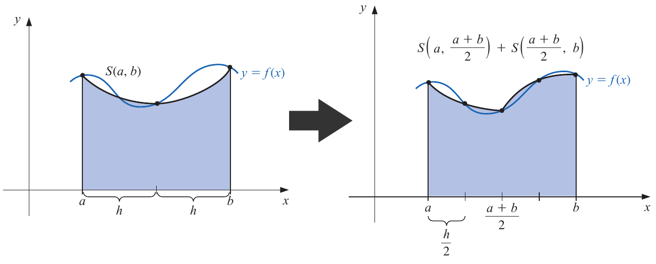
Now, instead of using an unique Simpson's quadrature, we implement two, yielding:
$$\int_a^bf(x)dx = S\left(a,\frac{a+b}{2}\right) + S\left(\frac{a+b}{2},b\right) - \frac{1}{16}\left(\frac{h^5}{90}\right)f^{(4)}(\xi)$$For this expression, we reasonably assume an equal fourth-order derivative $f^{(4)}(\xi) = f^{(4)}(\xi_1) = f^{(4)}(\xi_2) $, where $\xi_1$ is the estimative for the first subtinterval (i.e. $\xi_1\in[a,(a+b)/2]$), and $\xi_2$ for the second one (i.e. $\xi_1\in[(a+b)/2, b]$).
As both expressions can approximate the real value of the integrate, we can equal them, obtaining:
$$\int_a^bf(x)dx = S(a,b) - \frac{h^5}{90}f^{(4)}(\xi) = S\left(a,\frac{a+b}{2}\right) + S\left(\frac{a+b}{2},b\right) - \frac{1}{16}\left(\frac{h^5}{90}\right)f^{(4)}(\xi)$$which leads us to a simple way to estimate the error without knowing the fourth-order derivative, i.e.
$$\frac{h^5}{90}f^{(4)}(\xi) = \frac{16}{15}\left| S(a,b) - S\left(a,\frac{a+b}{2}\right) - S\left(\frac{a+b}{2},b\right) \right|$$If we fix a precision $\epsilon$, such that the obtained error for the second iteration is smaller
$$\frac{1}{16}\frac{h^5}{90}f^{(4)}(\xi) < \epsilon $$it implies:
$$\left| S(a,b) - S\left(a,\frac{a+b}{2}\right) - S\left(\frac{a+b}{2},b\right) \right|< 15 \epsilon$$and
$$\left| \int_a^bf(x) dx- S\left(a,\frac{a+b}{2}\right) - S\left(\frac{a+b}{2},b\right) \right|< \epsilon$$The second iteration is then $15$ times more precise than the first one.
Steps Simpson's adaptive quadrature
1. Give the function $f(x)$ to be integrated, the inverval $[a,b]$ and set a desired precision $\epsilon$.
2. Compute the next Simpsons's quadratures:
$$ S(a,b),\ S\left(a,\frac{a+b}{2}\right),\ S\left(\frac{a+b}{2},b\right) $$3. If
$$\frac{1}{15}\left| S(a,b) - S\left(a,\frac{a+b}{2}\right) - S\left(\frac{a+b}{2},b\right) \right|<\epsilon$$then the integration is ready and is given by:
$$\int_a^bf(x) dx \approx S\left(a,\frac{a+b}{2}\right) + S\left(\frac{a+b}{2},b\right) $$within the given precision.
4. If the previous step is not fulfilled, repeat from step 2 using as new intervals $[a,(a+b)/2]$ and $[(a+b)/2,b]$ and a new precision $\epsilon_1 = \epsilon/2$. Repeating until step 3 is fulfilled for all the subintervals.
Activity 
Models of Universe
From the Friedmann equations can be found the dynamics of the Universe, i.e., the evolution of the expansion with time that depends on the content of matter and energy of the Universe. Before introducing the general expression, there are several quatities that need to be defined.
It is convenient to express the density in terms of a critical density $\rho_c$ given by
\begin{equation} \rho_c = 3H_0^2/8\pi G \end{equation}where $H_o$ is the Hubble constant. The critical density is the density needed in order the Universe to be flat. To obtained it, it is neccesary to make the curvature of the universe $\kappa = 0$. The critical density is one value per time and the geometry of the universe depends on this value, or equally on $\kappa$. For a universe with $\kappa<0$ it would ocurre a big crunch(closed universe) and for a $\kappa>0$ there would be an open universe.
Now, it can also be defined a density parameter, $\Omega$, a normalized density
\begin{equation} \Omega_{i,0} = \rho_{i,0}/\rho_{crit} \end{equation}where $\rho_{i,0}$ is the actual density($z=0$) for the component $i$. Then, it can be found the next expression
\begin{equation} \frac{H^2(t)}{H_{0}^{2}} = (1-\Omega_0)(1+z)^2 + \Omega_{m,0}(1+z^3)+ \Omega_{r,0}(1+z)^4 + \Omega_{\Lambda,0} \end{equation}where $\Omega_{m,0}$, $\Omega_{r,0}$ and $\Omega_{\Lambda,0}$ are the matter, radiation and vacuum density parameters. And $\Omega_0$ is the total density including the vacuum energy.
This expression can also be written in terms of the expansion or scale factor($a$) rather than the redshift($z$) due to the expression $1+z = 1/a$ and it can be simplified in several ways.
For the next universe models, plot time($H_{0}^{-1}$ units) vs the scale factor:
-Einstein-de Sitter Universe: Flat space, null vacuum energy and dominated by matter
\begin{equation} t = H_0^{-1} \int_0^{a'} a^{1/2}da \end{equation}-Radiation dominated universe: All other components are not contributing
$$ t = H_0^{-1} \int_0^{a'} \frac{a}{[\Omega_{r,0}+a^2(1-\Omega_{r,0})]^{1/2}}da $$-WMAP9 Universe
\begin{equation} t = H_0^{-1} \int_0^{a'} \left[(1-\Omega_{0})+ \Omega_{m,0}a^{-1} + \Omega_{r,0}a^{-2} +\Omega_{\Lambda,0}a^2\right]^{-1/2} da \end{equation}You can take the cosmological parameters from the link
http://lambda.gsfc.nasa.gov/product/map/dr5/params/lcdm_wmap9.cfm or use these ones: $\Omega_M$ = 0.266, $\Omega_R = 8.24e-5$ and $\Omega_L = 0.734$.
Use composite simpson rule to integrate and compare it with the analitical expression in case you can get it. The superior limit in the integral corresponds to the actual redshift $z=0$. What is happening to our universe?
Activity 
Activity 
These integrals cannot be solved using analitical methods. Using the previous routine for adaptive quadrature, compute the integrals with a precision of $\epsilon=10^{-4}$ for values of $t=0.1,0.2,0.3,\cdots 1.0$. Create two arrays with those values and then make a plot of $c(t)$ vs $s(t)$. The resulting figure is called Euler spiral, that is a member of a family of curves called Clothoid loops.
Improper Integrals
Although the previous integration methods can be applied in almost every situation, improper integrals pose a challenger to numerical methods as they involve indeterminations and infinite intervals. Next, we shall cover some tricks to rewrite improper integrals in terms of simple ones.
Left endpoint singularity
Assuming a function $f(x)$ such that it can be rewritten as
$$ f(x) = \frac{g(x)}{(x-a)^p} $$the integral over an interval $[a,b]$ converges only and only if $0<p<1$.
Using Simpson's composite rule, it is possible to compute the fourth-order Taylor polynomial of the function $g(x)$ at the point $a$, obtaining
$$ P_4(x) = g(a) + g^{'}(a)(x-a)+\frac{g^{''}(a)}{2!}(x-a)^2 +\frac{g^{''}(a)}{3!}(x-a)^3+ \frac{g^{(4)}(a)}{4!}(x-a)^4$$The integral can be then calculated as
$$\int_a^b f(x)dx = \int_a^b\frac{g(x)-P_4(x)}{(x-a)^p}dx + \int_a^b\frac{P_4(x)}{(x-a)^p}dx$$The second term is an integral of a polynimal, which can be easily integrated using analytical methods.
The first term is no longer pathologic as there is not any indetermination, and it can be determined using composite Simpson's rule
Right endpoint singularity
This is the contrary case, where the indetermination is present in the extreme $b$ of the integration interval $[a,b]$. For this problem is enough to make a variable substitution
$$ z=-x \ \ \ \ \ \ dz=-dx$$With this, the right endpoint singularity becomes a left endpoint singularity and the previous method can be directly applied.
Infinite singularity
Finally, infinite singularities are those where the integration domain is infinite, i.e.
$$\int_a^\infty f(x)dx$$this type of integrals can be easily turned into a left endpoint singularity jus making the next variable substitution
$$t = x^{-1}\ \ \ \ \ dt = -x^{-2}dx$$yielding
$$ \int_a^\infty f(x)dx = \int_0^{1/a}t^{-2}f\left(\frac{1}{t}\right)dt $$Activity 
Using the substitution $u=t^2$ it is possible to use the previous methods for impropers integrals in order to evaluate the error function. Create a routine called ErrorFunction that, given a value of $x$, return the respective value of the integral.