
PLOTLY MATLAB API
WELCOME! This Notebook is designed to demonstrate the use of the Plotly MATLAB API and to showcase three **\*NEW\*** API functions:
fig2plotly.m
** • **getplotlyfig.m
** • **saveplotlyfig.m
New to Plotly?
Plotly is a browser-based data analysis and visualization tool that lets you and your team make and share beautiful, interactive graphs, 3D graphs, and streaming graphs using MATLAB, Python, IPython, matplotlib, R, ggplot2, and Excel.
This API allows MATLAB users to generate Plotly graphs from the desktop MATLAB environment: turning MATLAB figures into interactive, shareable, collaborative projects.
Plotly MATLAB API Workflow:
Collect or generate some data in your MATLAB environment
Send data to your Plotly account through this Plotly MATLAB API
View interactive graph in your browser
Style graph in the Plotly GUI
Share graph by URL shortlinks, Facebook, or Twitter
Export to PNG, PDF, EPS, SVG
***NEW* Plot your MATLAB figure objects with Plotly using fig2plotly.m**
***NEW* Get data, style, and layout from the plots stored online getplotlyfig.m**
***NEW* Save your Plotly figures as an image in MATLAB using saveplotlyfig.m**
Initial Setup:
The Plotly MATLAB API has been embedded into our MATLAB toolboxes and our Plotly credentials have been saved using plotlysetup.m. In order to start using the Plotly MATLAB API all we have to do now is start MATLAB! More information regarding installation / setting up the Plotly MATLAB API can be found on the online documentation.
NOTE: Throughout this notebook we will be using the super awesome pymatbridge package to communicate with MATLAB from Python. Everything that comes below the %%matlab decorator will now be read as MATLAB code. To use the MATLAB API on your own machine, simply open the MATLAB application as you normally would.
>> OPEN YOUR MATLAB ENVIRONMENT!
%load_ext pymatbridge
Starting MATLAB on ZMQ socket ipc:///tmp/pymatbridge
Send 'exit' command to kill the server
.MATLAB started and connected!
fig2plotly.m
Plot a MATLAB figure object with Plotly
***NEW*** to the Plotly MATLAB API is the fig2plotly.m function - the future of the MATLAB API. fig2plotly.m allows you to take your MATLAB generated figures and automatically create a Plotly plot, taking care of the conversion from the MATLAB figure object structure to Plotly syntax.
[INPUT]:
>> resp = fig2plotly()
>> resp = fig2plotly(f)
>> resp = fig2plotly(gcf)
>> resp = fig2plotly(f,'property',value, ... )
>> resp = fig2plotly(gcf,'property',value, ... )
**
[WHERE]:
**gcf - root figure object handle [double].
f - root figure object [struct] >> f = get(gcf)
**
[PROPERTIES]:
**'name' - name of the plot [string]['untitled']
'strip' - use plotly default styling [boolea][0]
'open' - opens a browser with plot result [boolean][1]
[OUTPUT]:
resp - results info of the plot [struct]
resp.[url,warning,message,filename,error]
If you are properly signed up / in, the url field of the structure array, resp, will contain the address (associated with your Plotly account) of your newly created Plotly plot. The filename field will return a string of your chosen file name, or 'untitled' by default. The warning, message, and error fields will contain a string if anything went wrong or if there are updates for the Plotly MATLAB API.
Example 1: fig2plotly.m
The best way to grasp the fig2plotly.m useage is to see it in action! For our first example, let's take a look at a plot featured in the Mathworks plot gallery.
%%matlab

%%%%%%%%%%%%%%%%%%%%%%%%%%%%%%%%%%%%%%%%%%%%%%%%%%%%
%            FROM MATLAB PLOT GALLERY              %
%  http://www.mathworks.com/discovery/gallery.html %
%%%%%%%%%%%%%%%%%%%%%%%%%%%%%%%%%%%%%%%%%%%%%%%%%%%%

api_path = ('/Users/chuckbronson/Documents/PLOTLY/MATLAB_API_REPO/DEV/TEST_PLOTS');
addpath(genpath(api_path));

load fitdata x y yfit;
fig = figure;
scatter(x, y, 'k');
line(x, yfit, 'color', 'k', 'linestyle', '-', 'linewidth', 2);
line(x, yfit + 0.3, 'color', 'r', 'linestyle', '--', 'linewidth', 2);
line(x, yfit - 0.3, 'color', 'r', 'linestyle', '--', 'linewidth', 2);
legend('Data', 'Localized Regression', 'Confidence Intervals', 2);
xlabel('X');
ylabel('Noisy');

%%%%%%%%%%%%%%%%%%%%%%%%%%%%%%%
%            PLOTLY           %
%%%%%%%%%%%%%%%%%%%%%%%%%%%%%%%

resp = fig2plotly(fig,'name','matlab_overview_1'); % <---- ONE LINE OF PLOTLY CODE!

The above plot is the ouptut from calling the scatter.m and line.m functions inherent in MATLAB. Using the fig2plotly.m function, we are able to extract the relevant data from the MATLAB figure object and throw the output over to our Plotly account! The returned response variable, resp, is a structure array which contains a url field with the address of our plot.
%%matlab
resp.url
ans =

https://plot.ly/~matlab_user_guide/661
Let's have a look at the newly produced line and scatter plot in Plotly!
NOTE: The following function can be used to embed your Plotly plots within your own NB.
from IPython.display import HTML

def show_plot(url, width=800, height=650):
    s = '<iframe height="%s" id="igraph" scrolling="no" frameborder = 0 seamless="seamless" src="%s" width="%s"></iframe>' %\
    (height, "/".join(map(str,[url, width, height])), width)
    return HTML(s)
show_plot('https://plot.ly/~matlab_user_guide/661')
Nice! We can see how the fig2plotly.m function is able to parse all the relevant information for the MATLAB figure object and generate an awesome looking plot, the data for which is now stored on the cloud! This means you'll never have to worry about where your data is saved on your computer and you can share your newly created plot by simply embedding the link within your website or throwing it over to Facebook or Twitter!
Another great thing about Plotly is the interactivity of the graphs. Try scrolling over the newly created plot to view the labelled data. Holding shift while clicking and dragging allows you to pan. Click and drag to zoom and double click to revert back to the original view.
We can also now take advantage of the interactive web app! You can view/edit all our newly created plots on your online account. By default fig2plotly.m will open your default browser and load your Plotly account to view the newly created plot. All the data associated with the plot has been conveniently stored in a spreadsheet that can be accessed by clicking on the the "View data" link on the right (image below).

By clicking on the "Save & edit" link on the left (image above), we are able to access the main web GUI. This will allow us to tweak and experiment with plotting layout and style without having to write lines upon lines of code. Below is a screen shot of the Plotly web app.

There are also many style/layout themes to choose from and you can even save your own themes to apply to your graphs. Have a go at changing the syle and layout to suit your personal preferences. Here is one that we made:
show_plot('https://plot.ly/~matlab_user_guide/662')
Once you are finished you can quickly share by hitting "Share". This will open a "Sharing settings" window (image below) which will allow you to modify the plots privacy settings and add a collaborator to be able to edit the plot you have created!

You can also click on the social media icons to quickly throw your plot over to Facebook or Twitter to share it with the world!
Example 2: fig2plotly.m
Lets have a look at how fig2plotly.m is able to handle more difficult plot layouts, such as multiple subplots of varying size.
%%matlab

%%%%%%%%%%%%%%%%%%%%%%%%%%%%%%%%%%%%%%%%%%%%%%%%%%%%
%            FROM MATLAB PLOT GALLERY              %
%  http://www.mathworks.com/discovery/gallery.html %
%%%%%%%%%%%%%%%%%%%%%%%%%%%%%%%%%%%%%%%%%%%%%%%%%%%%

fm = 20e3;
fc = 100e3;
tstep = 100e-9;
tmax  = 200e-6;
t = 0:tstep:tmax;
xam = (1 + cos(2*pi*fm*t)).*cos(2*pi*fc*t);
T = 1e-6;
N = 200;
nT = 0:T:N*T;
xn = (1 + cos(2*pi*fm*nT)).*cos(2*pi*fc*nT);
fig = figure;
subplot(2, 2, [1 3]);
plot(nT,xn);
xlabel('t');
ylabel('x[n]');
title('Sampled Every T=1e-6 ');
subplot(2, 2, 2);
plot(t, xam);
axis([0 200e-6 -2 2]);
title('AM Modulated Signal');
subplot(2, 2, 4);
plot(nT, xn);
title('Reconstruction at T=4e-6 ');

%%%%%%%%%%%%%%%%%%%%%%%%%%%%%%%
%           PLOTLY            %
%%%%%%%%%%%%%%%%%%%%%%%%%%%%%%%

resp = fig2plotly(fig,'strip',1,'name','matlab_overview_3');

Nice MATLAB! Now let's have a look at our newly generated Plotly plot.
show_plot('https://plot.ly/~matlab_user_guide/663')
Cool! fig2plotly.m preserves the subplot layout structure. It also converts the x-axis labels using the concise SI prefix μ = 10-6. You might notice that the colours for the traces generated using fig2plotly.m did not stay blue like the original output from MATLAB. This is because we changed the "strip" property of fig2plotly.m from "false" (default) to "true". In doing so we told fig2plotly.m to change the style used in MATLAB to Plotly's beautiful default color schemes.
Example 3A: fig2plotly.m
Now let's have a look at some other chart types in MATLAB and apply fig2plotly.m. Let's experiment with bar charts with a double y axis.
%%matlab

%%%%%%%%%%%%%%%%%%%%%%%%%%%%%%%%%%%%%%%%%%%%%%%%%%%%
%            FROM MATLAB PLOT GALLERY              %
%  http://www.mathworks.com/discovery/gallery.html %
%%%%%%%%%%%%%%%%%%%%%%%%%%%%%%%%%%%%%%%%%%%%%%%%%%%%

TBdata = [1990 4889 16.4; 1991 5273 17.4; 1992 5382 17.4; 1993 5173 16.5;
          1994 4860 15.4; 1995 4675 14.7; 1996 4313 13.5; 1997 4059 12.5;
          1998 3855 11.7; 1999 3608 10.8; 2000 3297  9.7; 2001 3332  9.6;
          2002 3169  9.0; 2003 3227  9.0; 2004 2989  8.2; 2005 2903  7.9;
          2006 2779  7.4; 2007 2725  7.2];

years = TBdata(:,1);
cases = TBdata(:,2);
rate  = TBdata(:,3);
fig = figure;
[ax, h1, h2] = plotyy(years, cases, years, rate, 'bar', 'plot');
set(h1, 'FaceColor', [0.8, 0.8, 0.8]);
set(h2, 'LineWidth', 2);
title('Tuberculosis Cases: 1991-2007');
xlabel('Years');
set(get(ax(1), 'Ylabel'), 'String', 'Cases');
set(get(ax(2), 'Ylabel'), 'String', 'Infection rate in cases per thousand');

%%%%%%%%%%%%%%%%%%%%%%%%%%%%%%%
%           PLOTLY            %
%%%%%%%%%%%%%%%%%%%%%%%%%%%%%%%

filename = 'matlab_overview_4';
resp = fig2plotly(fig,'name',filename);

The above plot is the ouptut we receive from calling the plotyy.m function inherent in MATLAB. Now, Let's grab that url from the resp structure aray and have a look at our newly genereted plot using fig2plotly.m.
%%matlab

resp.url
ans =

https://plot.ly/~matlab_user_guide/664
show_plot('https://plot.ly/~matlab_user_guide/664')
Sweet! Now we can use the Plotly web app to customize style an layout to our personal preference.
Alternatively... we can use the Plotly declaritive syntax to edit the style and layout with plotly.m, one of the original API functions. To do this, we will need to use another ***NEW*** function that simplifies everything: getplotlyfig.m.
getplotlyfig.m
Get data, style, and layout from the plots stored online
One of Plotly's secret powers is the ability to translate between MATLAB's structure/cell array syntax and JSON. This allows a smooth transition between the your figures in MATLAB and those stored in your Plotly account. In order to grab the data, style, and layout information from your plots living online, we've introduce a ***NEW*** funtion into the API: getplotlyfig.m. In fact, we can go one step further: getploylyfig.m lets you grab the data, style and layout of anyone's Plotly plots (as long as they are made public) - not just your own! See a graph you like online? Grab the data, style and layout and make one for yourself.
**[INPUT]:**
>> plotlyfigure = fig2plotly(file_owner,file_id)
**[WHERE]:**
file_owner - user name associated with the plot [string].
file_id - number identifier associated with the plot [string]
**[OUTPUT]:**
plotlyfigure - results info of the plot [struct]
plotlyfigure.[data,layout]
If the provided input arguments are valid, getplotlyfig.m returns a figure structure with data and layout fields. The data field is a cell array containing the exact same data, and style information as is required for the plotly.m function input. Likewise, the layout structure array contains all the layout information in the same form as is required for the plotly.m function input.
Example 3B: getplotlyfig.m
Now that we have a basic understanding of getplotlyfig.m, let's have a go at changing the bar and line colours from our previous example!
%%matlab

%%%%%%%%%%%%%%%%%%%%%%%%%%%%%%%
%       GET PLOTLY FIG!       %
%%%%%%%%%%%%%%%%%%%%%%%%%%%%%%%

plotlyfigure = getplotlyfig('bronsolo','82');


%%%%%%%%%%%%%%%%%%%%%%%%%%%%%%%
%         DATA/STYLE          %
%%%%%%%%%%%%%%%%%%%%%%%%%%%%%%%

% COLOUR CHOICES
col1 = '#3C8A22';
col2 = '#097054';
col3 = 'black';

% BAR CHART STYLE
plotlyfigure.data{1}.marker.color = col1;
plotlyfigure.data{1}.marker.line.width = 2;
plotlyfigure.data{1}.marker.line.color = col3;
plotlyfigure.data{1}.opacity = 0.7;
plotlyfigure.data{1}.name = 'Cases';

% LINE STYLE
plotlyfigure.data{2}.line.width = 10;
plotlyfigure.data{2}.line.color = col2;
plotlyfigure.data{2}.opacity = 0.7;
plotlyfigure.data{2}.name = 'Infection Rate';


%%%%%%%%%%%%%%%%%%%%%%%%%%%%%%%
%           LAYOUT            %
%%%%%%%%%%%%%%%%%%%%%%%%%%%%%%%

% Y2 AXIS STYLE
plotlyfigure.layout.yaxis2.titlefont.color = col3;
plotlyfigure.layout.yaxis2.tickfont.color = col2;
plotlyfigure.layout.yaxis2.tickcolor = col2;
plotlyfigure.layout.yaxis2.linecolor = col2;
plotlyfigure.layout.yaxis2.linewidth = 2;

% X AXIS STYLE
plotlyfigure.layout.xaxis.mirror = 0;
plotlyfigure.layout.xaxis.showline = 0;

% BAR LAYOUT
plotlyfigure.layout.bargap = 0.2;

%%%%%%%%%%%%%%%%%%%%%%%%%%%%%%%
%             ARGS            %
%%%%%%%%%%%%%%%%%%%%%%%%%%%%%%%

args.layout = plotlyfigure.layout;
args.filename = 'matlab_overview_5';
args.fileopt = 'new';


%%%%%%%%%%%%%%%%%%%%%%%%%%%%%%%
%           PLOTLY            %
%%%%%%%%%%%%%%%%%%%%%%%%%%%%%%%

resp = plotly(plotlyfigure.data,args);
url = resp.url
url =

https://plot.ly/~matlab_user_guide/775
show_plot('https://plot.ly/~matlab_user_guide/665')
Awesome! Note that we changed the names of the bar and line data so that when we scroll over the plot we get a nicely labeled interactive output. Give it a try!
Example 4: getplotlyfig.m
As we mentioned above, not only does getplotlyfig.m help us edit the plots that we made using fig2plotly.m, it also allows us to grab the data, style, and layout information from any public Plotly plot (say that three time fast) regardless of the API used to generate them. That means we can grab plots generated in R or Python and throw them into MATLAB to analyze, restyle, and throw back online. It's all the same to Plotly! Let's have a look at how that works. First, check out this sweet plot made by a user named "ReadtheBox".
show_plot('https://plot.ly/~ReadtheBox/35')
So sweet! Let's use getplotlyfig.m to grab the data/style and layout from this plot.
%%matlab

plotlyfigure = getplotlyfig('ReadtheBox','35') %grab the data from ReadtheBox (awesome Plotly user!)
plotlyfigure =

    layout: [1x1 struct]
      data: {1x9 cell}
Nice! Now let's have some fun changing things up. Let's have a look at the data field.
%%matlab

plotlyfigure.data{1}
ans =

    textfont: [1x1 struct]
        name: 'Runs'
      marker: [1x1 struct]
           y: [12 14 9 2 8 5 6 1 1 8 2 4 0 0]
           x: {1x14 cell}
        line: [1x1 struct]
        type: 'bar'
     error_y: [1x1 struct]
The data field is a {1x9} cell array where each element of the cell array corresponds to a different baseball statistic. The first data cell array element, plotlyfigure.data{1}, corresponds to the "Runs" data for each player.
Now, lets say we only wanted to look at "Runs" and "Hits". We can do that easily by grabbing the first two elements of the data cell array.
%%matlab

%%%%%%%%%%%%%%%%%%%%%%%%%%%%%%%
%         DATA/STYLE          %
%%%%%%%%%%%%%%%%%%%%%%%%%%%%%%%

traces= {plotlyfigure.data{1},plotlyfigure.data{2}}; % <--- FIRST TWO DATA ELEMENTS


%%%%%%%%%%%%%%%%%%%%%%%%%%%%%%%
%            ARGS             %
%%%%%%%%%%%%%%%%%%%%%%%%%%%%%%%

args.filename = 'matlab_overview_6';
args.fileopt = 'new';
args.layout = plotlyfigure.layout;

%%%%%%%%%%%%%%%%%%%%%%%%%%%%%%%
%           PLOTLY            %
%%%%%%%%%%%%%%%%%%%%%%%%%%%%%%%

resp = plotly(traces,args); % <--- USE PLOTLY TO THROW OUR NEW PLOT ONLINE
resp.url
ans =

https://plot.ly/~matlab_user_guide/776
Let's take a look:
show_plot('https://plot.ly/~matlab_user_guide/666')
Awesome - Go Ellsbury!
Now let's change some layout settings. How about we change the barmode from 'stack' to 'group'.
%%matlab

%%%%%%%%%%%%%%%%%%%%%%%%%%%%%%%
%         DATA/STYLE          %
%%%%%%%%%%%%%%%%%%%%%%%%%%%%%%%

traces= {plotlyfigure.data{1},plotlyfigure.data{2}}; % <--- FROM BEFORE!


%%%%%%%%%%%%%%%%%%%%%%%%%%%%%%%
%           LAYOUT            %
%%%%%%%%%%%%%%%%%%%%%%%%%%%%%%%

plotlyfigure.layout.barmode = 'group';  % <--- CHANGE FROM STACK TO GROUP!


%%%%%%%%%%%%%%%%%%%%%%%%%%%%%%%
%             ARGS            %
%%%%%%%%%%%%%%%%%%%%%%%%%%%%%%%

% ARGS STRUCTURE
args.filename = 'matlab_overview_7';
args.fileopt = 'new';
args.layout = plotlyfigure.layout;


%%%%%%%%%%%%%%%%%%%%%%%%%%%%%%%
%           PLOTLY            %
%%%%%%%%%%%%%%%%%%%%%%%%%%%%%%%

resp = plotly(traces,args);
resp.url
ans =

https://plot.ly/~matlab_user_guide/777
show_plot('https://plot.ly/~matlab_user_guide/669')
Cool!
But... what happens if we want to put our graph in a report or thesis? So far all we have seen is how to share/embed our plots online. What we need now is to save our Plotly figures as images. For that we use the ***NEW*** saveplotlyfig.m function...
saveplotlyfig.m
Save your MATLAB figure as an image using Plotly
saveplotlyfig.m allows you to convert your MATLAB figures into static images using Plotly.
**[INPUT]:**
>> saveplotlyfig(data, filename)
>> saveplotlyfig(plotlyfigure, filename)
**[WHERE]:**
data - data/style of plot [cell array]
plotlyfigure.data - data/style of plot [cell array]
plotlyfigure.layout - layout of plot [struct]
filename - name of image to be saved [string]
**[OUTPUT]:**
PNG image 'filename' saved to your working directory
Currently saveplotlyfig.m supports PNG, PDF, JPEG, and SVG. If data, layout and filename are structure correctly, saveplotlyfig.m will automatically save the PNG image named 'filename' to your working directory.
EXAMPLE 5: saveplotlyfig.m
Let's have a look at saveplotlyfig.m to see how it works. Check out this next plot that was featured on the MATLAB plot gallery.
%%matlab

%%%%%%%%%%%%%%%%%%%%%%%%%%%%%%%%%%%%%%%%%%%%%%%%%%%%
%            FROM MATLAB PLOT GALLERY              %
%  http://www.mathworks.com/discovery/gallery.html %
%%%%%%%%%%%%%%%%%%%%%%%%%%%%%%%%%%%%%%%%%%%%%%%%%%%%

% Load Morse data
load MDdata dissimilarities dist1 dist2 dist3

% Plot the first set of data in blue
fig = figure;
plot(dissimilarities, dist1, 'bo');
hold on;

% Plot the second set of data in red
plot(dissimilarities, dist2, 'r+');

% Plot the third set of data in green
plot(dissimilarities, dist3, 'g^');

% Add title and axis labels
title('Morse Signal Analysis');
xlabel('Dissimilarities');
ylabel('Distances');


%%%%%%%%%%%%%%%%%%%%%%%%%%%%%%%
%            PLOTLY           %
%%%%%%%%%%%%%%%%%%%%%%%%%%%%%%%

filename = 'matlab_overview_8';
resp = fig2plotly(fig,'name',filename);

%%matlab

resp.url
ans =

https://plot.ly/~matlab_user_guide/670
Good job MATLAB - let's look at the Plotly graph we created!
show_plot('https://plot.ly/~matlab_user_guide/670')
So awesome! Now let's save this plot as a PNG image using **saveplotlyfig.m**.
%%matlab

%%%%%%%%%%%%%%%%%%%%%%%%%%%%%%%
%       GET PLOTLY FIG!       %
%%%%%%%%%%%%%%%%%%%%%%%%%%%%%%%

plotlyfigure = getplotlyfig('matlab_user_guide','670');

%%%%%%%%%%%%%%%%%%%%%%%%%%%%%%%
%      SAVE PLOTLY FIG!       %
%%%%%%%%%%%%%%%%%%%%%%%%%%%%%%%

filename = 'morse.png';

saveplotlyfig(plotlyfigure,filename)
Boom! **morse.png** has been automatically saved to our working directory. Let's have a look.

Awesome! Do you notice how the above plot is no longer interactive? That's because it is a static PNG image, ready to be placed in your offline documents.
Plotly graphics are rendered as high-quality vector graphics so they embed really well in presentations and reports.
Take a look for yourself. Here are the static image versions of the following plot.
show_plot('https://plot.ly/~chris/1638/')
Example 6: saveplotlyfig.m
As a final example, let's grab a public plot from another Plotly user. This one is an awesome line plot from our very own jackp.
show_plot('https://plot.ly/~jackp/671')
First grab the data/style and layout.
%%matlab

plotlyfig = getplotlyfig('jackp','671')
plotlyfig =

    layout: [1x1 struct]
      data: {1x11 cell}
Now feed the data/style and layout information into saveplotlyfig.m.
%%matlab
filename = 'tax.png';
saveplotlyfig(plotlyfig,filename);
Cool! Let's have a look at the image.
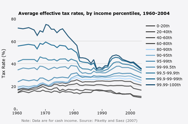
All we have to do now is throw it into our economics report!
CONTACT
Want to help improve this notebook? Please send us your comments/questions! Feedback concerning this notebook can be directed to ** chuck [at] plot.ly **. You can also follow us online.


** • **
** • **
** • **
** • **
** • **
** • **
** • **
NOTEBOOK BEAUTIFICATION
# CSS styling within IPython notebook
from IPython.core.display import HTML
def css_styling():
    styles = open("./css/style_notebook.css", "r").read()
    return HTML(styles)

css_styling()