Introduction to NumPy
- Jake VanderPlas
- Presented at PyData @ Strata, New York City
- October 15, 2014
The source for this notebook can be found at http://github.com/jakevdp/PyData2014
NumPy is a huge project, and there's no way to give a complete picture of it in ~40 minutes. So the goal today is to give a motivation for NumPy and a quick intro to what you'll need to get started.
Note that this tutorial is written for Python 3.3 or newer. In order to be compatible with Python 2.x, we'll do some __future__ imports to start off:
from __future__ import print_function, division
Outline
- Motivating NumPy: it increases both coding efficiency and computational efficiency
- Why is NumPy Faster than Python?
- The core of it all: the ndarray
- Universal Functions
- Aggregates
Motivating NumPy: Efficient Numerical Computing
We'll start by attempting to motivate why you might want to use NumPy for numerical code. Suppose you'd like to use a plotting tool to graph $y = \sin(x)$ for $0 \le x \le 2\pi$. Let's think about how you might do this in Python.
We'll briefly preview matplotlib for plotting here; more on this later!
%matplotlib inline
import matplotlib.pyplot as plt

# Setup ggplot style, if using matplotlib 1.4 or newer
try:
    plt.style.use('ggplot')
    print("Setting Matplotlib style to ggplot")
except AttributeError:
    print("Update matplotlib to enable styles")
Setting Matplotlib style to ggplot
First Try: A C-like Approach
A new Python user with a background in a low-level language like C or Fortran might approach the problem this way:
import math
xmin = 0
xmax = 2 * math.pi
N = 1000
# build the arrays
x = []
y = []
for i in range(N):
    xval = xmin + i * (xmax - xmin) / N
    x.append(xval)
    y.append(math.sin(xval))

# Plot the result with matplotlib
plt.plot(x, y);

The C/Fortran approach is very prodecural, low-level, and "hands-on". Our program individually creates and modifies every value in each list.
Second Try: A "Pythonic" Approach
A more "Pythonic" approach would be to avoid the loops in favor of constructs like list or generator comprehensions. A Python expert without too much numerical background might proceed like this:
x = [xmin + i * (xmax - xmin) / N for i in range(N)]
y = [math.sin(xi) for xi in x]

plt.plot(x, y);
The Pythonic approach is beautiful, in that the lists are created in terse yet easy to grok one-line statements.
Third Try: a NumPy Approach
import numpy as np

x = np.linspace(xmin, xmax, N)
y = np.sin(x)

plt.plot(x, y);

The NumPy version is perhaps the simplest of all: instead of setting each element of each array "by hand", as it were, we instead use simple functions which will create arrays and operate on them element-wise.
Let's look at all these side-by-side:
#---------------------------------------------------
# 1. C/Fortran style
x = []
y = []
for i in range(N):
    xval = xmin + i * (xmax - xmin) / N
    x.append(xval)
    y.append(math.sin(xval))

#---------------------------------------------------
# 2. Pythonic approach
x = [xmin + i * (xmax - xmin) / N for i in range(N)]
y = [math.sin(xi) for xi in x]

#---------------------------------------------------
# 3. NumPy approach
x = np.linspace(xmin, xmax, N)
y = np.sin(x)
It's clear that NumPy is the most efficient to type; how does it compare when it comes to computation time? Let's use IPython's %%timeit cell magic to check. To make things more interesting, let's increase N to 100,000:
N = 100000
%%timeit
# 1. C/Fortran style
x = []
y = []
for i in range(N):
    xval = xmin + i * (xmax - xmin) / N
    x.append(xval)
    y.append(math.sin(xval))
10 loops, best of 3: 61.2 ms per loop
%%timeit
# 2. Pythonic style
x = [xmin + i * (xmax - xmin) / N for i in range(N)]
y = [math.sin(xi) for xi in x]
10 loops, best of 3: 45.3 ms per loop
%%timeit
# 3. NumPy approach
x = np.linspace(xmin, xmax, N)
y = np.sin(x)
1000 loops, best of 3: 1.74 ms per loop
We see that for this operation, NumPy is 30-40x faster than either of the pure Python approaches!
What we've seen above, in a nutshell, is why NumPy is useful for numerical computing:
- Numerical operations across arrays are faster and more natural to type.
- Numerical operations across arrays are more clear to read.
- Numerical operations across arrays are more computationally efficient.
So Why is NumPy So Much Faster?
The reasons that these operations are so much faster in NumPy than in Python boils down to the fact that Python is not a compiled language, while NumPy pushes certain operations down into compiled code. We'll talk about three main components of this below:
1. Python is Dynamically rather than Statically Typed
Python is a dynamically-typed language, where just about anything goes. This means you can do things that would seem downright silly in C or Fortran, like replace an integer in an array with a string:
L = list(range(5))
L
[0, 1, 2, 3, 4]
L[3] = "three"
L
[0, 1, 2, 'three', 4]
The reason that Python can be so flexible is that, fundamentally all objects are of the same type: they are PyObject instances. Each PyObject does have an indicator of what type it is, but this information is accessed at run-time, rather than at some compile phase.
Functionally, the difference between a C integer and a Python integer looks like this:
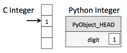
That PyObject_HEAD block is what contains all of Python's dynamic goodies, like the type, reference count, etc.
Yes, there are modern JIT-compiled languages which bridge this gap, but Python doesn't yet do this, and the projects that do (PyPy, Pyston, etc.) aren't yet mature enough to use for numerical computing in practice.
2. Python is Interpreted rather than Compiled
This dynamic type-checking means that Python's code cannot be pre-compiled, as with C/Fortran/etc. So, for example, when we multiply each of our list elements by two, we get the following:
[2 * Li for Li in L]
[0, 2, 4, 'threethree', 8]
Notice that the * operator does fundamentally different things with integer vs. string objects!
Here the * cannot be mapped onto some machine-code function until the program is actually run: this leads to type-checking overhead each time the function is called, even if you have an array of all integers! There's no way for Python to know ahead of time that the same * needs to be used each time: this is the sense in which it's interpreted rather than compiled.
Yes, Python is compiled to a sort of bytecode (i.e. .pyc files), but no deep optimization takes place: this bytecode is basically a 1-to-1 mapping to the Python code that generates it.
3. Python's flexible object model can lead to inefficiencies
When it comes to creating lists or arrays of objects, the fact that Python is dynamically typed can make a huge difference: consider the memory layout of a NumPy array vs that of a Python list. Consider the following two objects:
L = list(range(1, 9))
L
[1, 2, 3, 4, 5, 6, 7, 8]
A = np.arange(1, 9)
A
array([1, 2, 3, 4, 5, 6, 7, 8])
They may look superfically similar, but under the hood they are anything but. Here's a schematic of their memory configuration under-the-hood:
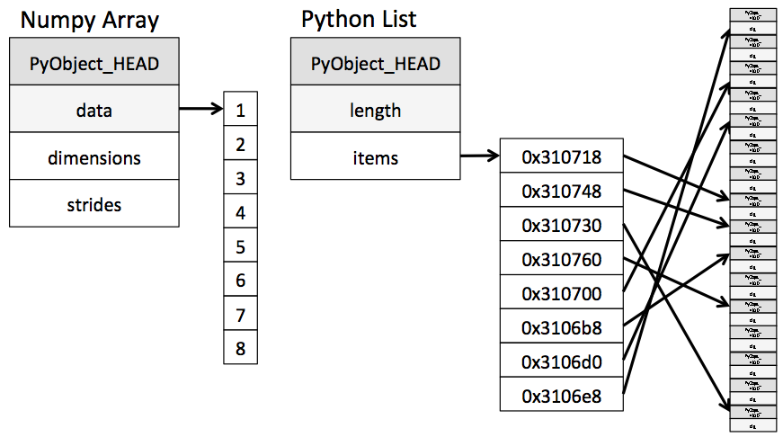
NumPy arrays are simply pointers to buffers containing data of a uniform type; Python lists are pointers to pointers, each of which in turn points to a PyObject instance existing in memory.
Yes, Python has built-in array objects that provide mono-typed storage buffers, but they are nowhere near as useful as NumPy's arrays.
Exploring NumPy's ndarray object
NumPy's ndarray object is essentially a pointer to a data buffer, with metadata telling us how to interpret it.
For example, we can create the following one-dimensional array:
x = np.arange(10)
x
array([0, 1, 2, 3, 4, 5, 6, 7, 8, 9])
Let's look at some of the important attributes of this object:
# data type
x.dtype
dtype('int64')
# array shape
x.shape
(10,)
# number of dimensions
x.ndim
1
# size of the array
x.size
10
# number of bytes to step for each dimension
x.strides
(8,)
# flags specifying array properties
x.flags
  C_CONTIGUOUS : True
  F_CONTIGUOUS : True
  OWNDATA : True
  WRITEABLE : True
  ALIGNED : True
  UPDATEIFCOPY : False
Arrays as Views
Let's focus on this OWNDATA property of the x array above.
Here we see that the array x owns its data, but if we create some derived array from x, this will change.
Let's use Python's standard slicing syntax to create a new array containing every other item in x:
y = x[::2]
y
array([0, 2, 4, 6, 8])
Checking y's flags, we see now that OWNDATA is False:
y.flags
  C_CONTIGUOUS : False
  F_CONTIGUOUS : False
  OWNDATA : False
  WRITEABLE : True
  ALIGNED : True
  UPDATEIFCOPY : False
x still owns the data; y simply has a pointer to it!
Let's demonstrate this by changing one of the values in y, and observing that the corresponding x value changes as well:
y[2] = 100
x
array([ 0, 1, 2, 3, 100, 5, 6, 7, 8, 9])
So how does this work?
It turns out that x and y point to the same memory buffer, but view it in different ways:
import ctypes
print(x.data, x.itemsize, x.strides)
print(y.data, y.itemsize, y.strides)
<memory at 0x106b72c80> 8 (8,)
<memory at 0x106b72c80> 8 (16,)
The strides attribute shows you the number of bytes for each step in the array; y essentially takes two 8-byte steps each time it accesses the next array element.
print(x)
print(y)
[  0   1   2   3 100   5   6   7   8   9]
[  0   2 100   6   8]
Thus we see that when constructing arrays, we generally will end up with views rather than copies of source arrays. This is one extremely powerful aspect of NumPy, but also something you should certainly be aware of!
# Side note: if you actually want a copy, you can do, e.g.
y = x[::2].copy()
Such views can be even more powerful: for example, we can reshape x into a two-dimensional array:
x2 = x.reshape(2, 5)
x2
array([[  0,   1,   2,   3, 100],
       [  5,   6,   7,   8,   9]])
Again, this is simply a view of x:
x2[1, 4] = 42
x2
array([[  0,   1,   2,   3, 100],
       [  5,   6,   7,   8,  42]])
x
array([ 0, 1, 2, 3, 100, 5, 6, 7, 8, 42])
Let's see some of the attributes of x2:
# number of dimensions
x2.ndim
2
# shape of the array
x2.shape
(2, 5)
# size of the array
x2.size
10
# number of bytes to step for each dimension
x2.strides
(40, 8)
x2.flags
  C_CONTIGUOUS : True
  F_CONTIGUOUS : False
  OWNDATA : False
  WRITEABLE : True
  ALIGNED : True
  UPDATEIFCOPY : False
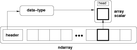
So as you use NumPy arrays, keep this in mind! What you are using is a Python object which views a raw data buffer as a flexible array:
Creating NumPy Arrays
Here we'll demonstrate some functions to create NumPy arrays from scratch:
# Array of zeros
np.zeros((2, 3))
array([[ 0.,  0.,  0.],
       [ 0.,  0.,  0.]])
# Array of ones
np.ones((3, 4))
array([[ 1.,  1.,  1.,  1.],
       [ 1.,  1.,  1.,  1.],
       [ 1.,  1.,  1.,  1.]])
# Like Python's range() function
np.arange(10)
array([0, 1, 2, 3, 4, 5, 6, 7, 8, 9])
# 5 steps from 0 to 1
np.linspace(0, 1, 5)
array([ 0. , 0.25, 0.5 , 0.75, 1. ])
# uninitialized array
np.empty(10)
array([ 0., 0., 0., 0., 0., 0., 0., 0., 0., 0.])
# random numbers between 0 and 1
np.random.rand(5)
array([ 0.48200098, 0.91255848, 0.43654199, 0.86788548, 0.36746416])
# standard-norm-distributed random numbers
np.random.randn(5)
array([-0.86029106, 0.27795606, -1.59104791, -0.30107627, 0.46938077])
Some Strategies for Fast Computing with NumPy
Here we'll discuss a couple strategies for fast computing with NumPy. In particular, we'll mention universal functions, which operate elementwise on arrays, and aggregate functions, which collapse arrays along particular dimensions.
Universal Functions
Where the rubber hits the road with NumPy is with Universal functions: these are functions which operate elementwise on arrays. We saw this above with the np.sin function, which takes an array and returns an array with the elementwise sine:
x = np.linspace(0, 2 * np.pi)
y = np.sin(x)
print(x.shape)
print(y.shape)
(50,)
(50,)
plt.plot(x, y);

NumPy also implements many arithmetic functions (e.g. +, -, *, /, **) as element-wise ufuncs. So we can do things like this:
plt.plot(x, y)
plt.plot(x, y + 1)
plt.plot(x, -2 * y)
plt.plot(x, 1 / (1 + y ** 2));

You can find a lot of interesting ufuncs in NumPy: for example
for f in [np.sin, np.cos, np.exp, np.log, np.sinc]:
    plt.plot(x, f(x), label='np.' + f.__name__)
plt.legend()
plt.ylim(-1, 5)
-c:2: RuntimeWarning: divide by zero encountered in log
(-1, 5)

Other interesting functions can be found in scipy.special. For example, here are some Bessell functions:
from scipy import special
x = np.linspace(0, 30, 500)
plt.plot(x, special.j0(x), label='j0')
plt.plot(x, special.j1(x), label='j1')
plt.plot(x, special.jn(3, x), label='j3')
plt.legend();

There are far, far more options available, and if you want some sort of specialized mathematical function, you can probably find a ufunc version of it in scipy.special.
Perhaps the best way to explore this is to use IPython's help or tab-completion features:
from scipy import special
special?
Notice the key here UFuncs loop over data for you, so you don't have to write these loops by hand in Python.
Aggregate Functions
Aggregate function are those which collapse an array along a particular dimension.
For example, the minimum of an array can be found using NumPy's min() aggregate:
x = np.random.random(100)
x.min()
0.0040929643153089224
Other aggregates exist as well:
# Maximum value
x.max()
0.96697914536521146
# Sum
x.sum()
49.430117531542443
# Mean
x.mean()
0.49430117531542445
# Product
x.prod()
4.6730597420222299e-46
# Standard Deviation
x.std()
0.28299025459860538
# Variance
x.var()
0.080083484197783508
# Median
np.median(x)
0.51601049164335466
# Quantiles
np.percentile(x, [25, 50, 75])
array([ 0.25034498, 0.51601049, 0.71508313])
For multi-dimensional arrays, we can compute aggregates along certain specified dimensions:
y = np.arange(12).reshape(3, 4)
y
array([[ 0,  1,  2,  3],
       [ 4,  5,  6,  7],
       [ 8,  9, 10, 11]])
# sum of each column
y.sum(0)
array([12, 15, 18, 21])
# sum of each row
y.sum(1)
array([ 6, 22, 38])
# Keep the dimensions (NumPy 1.7 or later)
y.sum(1, keepdims=True)
array([[ 6],
       [22],
       [38]])
np.std(y, 0)
array([ 3.26598632, 3.26598632, 3.26598632, 3.26598632])
As with ufuncs, the key is this: Aggregates loop over data for you, so you don't have to write the loops yourself in Python.
Last Thoughts; Where to Learn More
We've just scratched the surface here: there is much more to using NumPy effectively and efficiently. We haven't covered topics like advanced indexing & slicing, masked arrays, structured arrays, linear algebra, fourier transforms, and the many more utilities that are available.
If there's one thing to take away from this brief introduction, it's this:
If you write Python loops which scan over your data, you're (most likely) doing it wrong.
NumPy provides routines to replace loops with vectorized operations, as we've seen above, and this is where it gains its efficiency.
For a more in-depth presentiation on the subject of efficient computing with NumPy, you can see this 1.5 hour tutorial I gave at PyData 2013 (view the notebook here).