This notebook was put together by Jake Vanderplas for UW's Astro 599 course. Source and license info is on GitHub.
%run talktools.py
Efficient Numerical Computing with Numpy
In this session, we'll discuss how to make your programs as efficient as possible, mainly by taking advantage of vectorization in NumPy.
Aside: the "Unladen Swallow"
from IPython.display import YouTubeVideo
YouTubeVideo("y2R3FvS4xr4")
That video was the original reference behind the now-defunct unladen swallow project, which had the goal of making Python's C implementation faster.
Yes, Python is (unfortunately) a rather slow language.
Here is an example:
# A silly function implemented in Python

def func_python(N):
    d = 0.0
    for i in range(N):
        d += (i % 3 - 1) * i
    return d
# Use IPython timeit magic to time the execution
%timeit func_python(10000)
1000 loops, best of 3: 1.63 ms per loop
To compare to a compiled language, let's write the same function in fortran and use the f2py tool (included in NumPy) to compile it
%%file func_fortran.f

      subroutine func_fort(n, d)
           integer, intent(in) :: n
           double precision, intent(out) :: d
           integer :: i
           d = 0
           do i = 0, n - 1
                d = d + (mod(i, 3) - 1) * i
           end do
      end subroutine func_fort
Overwriting func_fortran.f
# use f2py rather than f2py3 for Python 2
!f2py3 -c func_fortran.f -m func_fortran > /dev/null
from func_fortran import func_fort
%timeit func_fort(10000)
100000 loops, best of 3: 15.7 µs per loop
Fortran is about 100 times faster for this task!
Why is Python so slow?
We alluded to this yesterday, but languages tend to have a compromise between convenience and performance.
C, Fortran, etc.: static typing and compiled code leads to fast execution
- But: lots of development overhead in declaring variables, no interactive prompt, etc.
Python, R, Matlab, IDL, etc.: dynamic typing and interpreted excecution leads to fast development
- But: lots of execution overhead in dynamic type-checking, etc.
We like Python because our development time is generally more valuable than execution time. But sometimes speed can be an issue.
Strategies for making Python fast
Use Numpy ufuncs to your advantage
Use Numpy aggregates to your advantage
Use Numpy broadcasting to your advantage
Use Numpy slicing and masking to your advantage
Use a tool like SWIG, cython or f2py to interface to compiled code.
Here we'll cover the first four, and leave the fifth strategy for a later session.
Strategy 1: Using UFuncs in Numpy
A ufunc in numpy is a Universal Function. This is a function which operates element-wise on an array. We've already seen examples of these in the various arithmetic operations:
import numpy as np
x = np.random.random(4)
print(x)
print(x + 1)  # add 1 to each element of x
[ 0.14407406  0.1104411   0.82417477  0.61817359]
[ 1.14407406  1.1104411   1.82417477  1.61817359]
x * 2 # multiply each element of x by 2
array([ 0.28814812, 0.22088221, 1.64834954, 1.23634718])
x * x # multiply each element of x by itself
array([ 0.02075734, 0.01219724, 0.67926405, 0.38213859])
x[1:] - x[:-1]
array([-0.03363296, 0.71373367, -0.20600118])
These are binary ufuncs: they take two arguments.
There are also many unary ufuncs:
-x
array([-0.14407406, -0.1104411 , -0.82417477, -0.61817359])
np.sin(x)
array([ 0.14357615, 0.11021673, 0.73398757, 0.57954772])
The Speed of Ufuncs
x = np.random.random(10000)
%%timeit
# compute element-wise x + 1 via a ufunc
y = np.zeros_like(x)
y = x + 1
10000 loops, best of 3: 21.1 µs per loop
%%timeit
# compute element-wise x + 1 via a loop
y = np.zeros_like(x)
for i in range(len(x)):
    y[i] = x[i] + 1
100 loops, best of 3: 3.43 ms per loop
Why is NumPy so much faster?
Numpy UFuncs are faster than Python functions involving loops, because the looping happens in compiled code. This is only possible when types are known beforehand, which is why numpy arrays must be typed.
x = np.random.random(5)
print(x)
print(np.minimum(x, 0.5))
print(np.maximum(x, 0.5))
[ 0.18846954  0.66824324  0.10376865  0.43608056  0.36835284]
[ 0.18846954  0.5         0.10376865  0.43608056  0.36835284]
[ 0.5         0.66824324  0.5         0.5         0.5       ]
# contrast this behavior with that of min() and max()
print(np.min(x))
print(np.max(x))
0.103768651674
0.668243237764
%matplotlib inline
# On older IPython versions, use %pylab inline
import matplotlib.pyplot as plt
x = np.linspace(0, 10, 1000)
plt.plot(x, np.sin(x));

from scipy.special import gammaln
plt.plot(x, gammaln(x));

Some interesting properties of UFuncs
UFuncs have some methods built-in, which allow for some very interesting, flexible, and fast operations:
x = np.arange(5)
y = np.arange(1, 6)
np.add(x, y)
array([1, 3, 5, 7, 9])
np.add.accumulate(x)
array([ 0, 1, 3, 6, 10])
np.multiply.accumulate(x)
array([0, 0, 0, 0, 0])
np.multiply.accumulate(y)
array([ 1, 2, 6, 24, 120])
np.add.identity
0
np.multiply.identity
1
np.add.outer(x, y)
array([[1, 2, 3, 4, 5],
       [2, 3, 4, 5, 6],
       [3, 4, 5, 6, 7],
       [4, 5, 6, 7, 8],
       [5, 6, 7, 8, 9]])
# make a times-table
x = np.arange(1, 13)
np.multiply.outer(x, x)
array([[  1,   2,   3,   4,   5,   6,   7,   8,   9,  10,  11,  12],
       [  2,   4,   6,   8,  10,  12,  14,  16,  18,  20,  22,  24],
       [  3,   6,   9,  12,  15,  18,  21,  24,  27,  30,  33,  36],
       [  4,   8,  12,  16,  20,  24,  28,  32,  36,  40,  44,  48],
       [  5,  10,  15,  20,  25,  30,  35,  40,  45,  50,  55,  60],
       [  6,  12,  18,  24,  30,  36,  42,  48,  54,  60,  66,  72],
       [  7,  14,  21,  28,  35,  42,  49,  56,  63,  70,  77,  84],
       [  8,  16,  24,  32,  40,  48,  56,  64,  72,  80,  88,  96],
       [  9,  18,  27,  36,  45,  54,  63,  72,  81,  90,  99, 108],
       [ 10,  20,  30,  40,  50,  60,  70,  80,  90, 100, 110, 120],
       [ 11,  22,  33,  44,  55,  66,  77,  88,  99, 110, 121, 132],
       [ 12,  24,  36,  48,  60,  72,  84,  96, 108, 120, 132, 144]])
Ufunc mini-exercises
Each of the following functions take an array as input, and return an array as output. They are implemented using loops, which is not very efficient.
For each function, implement a fast version which uses ufuncs to calculate the result more efficiently. Double-check that you get the same result for several different arrays.
use the %timeit magic to time the execution of the two implementations for a large array (say, 1000 elements).
# 1. computing the element-wise sine + cosine

from math import sin, cos
def slow_sincos(x):
    """x is a 1-dimensional array"""
    y = np.zeros_like(x)
    for i in range(len(x)):
        y[i] = sin(x[i]) + cos(x[i])
    return y

x = np.random.random(5)
print(slow_sincos(x))
[ 1.38638594 1.41068192 1.41074488 1.39904614 1.39058355]
# write a fast_sincos function
# 2. computing the difference between adjacent squares

def slow_sqdiff(x):
    """x is a 1-dimensional array"""
    y = np.zeros(len(x) - 1)
    for i in range(len(y)):
        y[i] = x[i + 1] ** 2 - x[i] ** 2
    return y

x = np.random.random(5)
print(slow_sqdiff(x))
[ 0.40936747 -0.30871454 0.49088252 -0.1586789 ]
# write a fast_sqdiff function
# 3. computing the outer-product of each consecutive pair

def slow_pairprod(x):
    """x is a 1-dimensional array"""
    if len(x) % 2 != 0:
        raise ValueError("length of x must be even")
    N = len(x) // 2
    y = np.zeros((N, N))
    for i in range(N):
        for j in range(N):
            y[i, j] = x[2 * i] * x[2 * j + 1]
    return y

x = np.arange(1, 9)
print(slow_pairprod(x))
[[  2.   4.   6.   8.]
 [  6.  12.  18.  24.]
 [ 10.  20.  30.  40.]
 [ 14.  28.  42.  56.]]
# write a fast_pairprod function
Strategy 2. Using Numpy Aggregates
Aggregates are functions over arrays which return smaller arrays.
Numpy has several built-in
# 10 x 10 array drawn from a standard normal
x = np.random.randn(10, 10)
x.mean()
0.0086655841045156605
np.mean(x)
0.0086655841045156605
x.std()
0.99647690340540895
x.var()
0.99296621902043269
x.sum()
0.86655841045156601
x.prod()
4.788617672159386e-22
np.median(x)
0.12432664008018213
np.percentile(x, 50)
0.12432664008018213
np.percentile(x, (25, 75))
array([-0.59558374, 0.6702099 ])
Aggregates along certain dimensions
x = np.random.rand(3, 5)
x
array([[ 0.90877938,  0.58853087,  0.3233339 ,  0.63680331,  0.64820305],
       [ 0.37713506,  0.68006887,  0.68975908,  0.53422032,  0.3331116 ],
       [ 0.93016689,  0.55381498,  0.35948829,  0.80807909,  0.34102259]])
x.sum(0) # sum all rows
array([ 2.21608134, 1.82241471, 1.37258128, 1.97910272, 1.32233723])
x.sum(1) # sum all columns
array([ 3.10565051, 2.61429493, 2.99257184])
np.median(x, 1)
array([ 0.63680331, 0.53422032, 0.55381498])
np.mean(x, 1)
array([ 0.6211301 , 0.52285899, 0.59851437])
Binary ufuncs as aggregates
Any binary ufunc (a ufunc taking two arguments) can be turned into an aggregate using the reduce() method:
np.sum(x, 1)
array([ 3.10565051, 2.61429493, 2.99257184])
np.add.reduce(x, 1)
array([ 3.10565051, 2.61429493, 2.99257184])
np.prod(x, 1)
array([ 0.07138309, 0.03148164, 0.05103256])
np.multiply.reduce(x, 1)
array([ 0.07138309, 0.03148164, 0.05103256])
np.divide.reduce(x, 1)
array([ 11.56968674, 4.51789808, 16.95408724])
A caution: for reduce methods, the default axis is 0:
np.add.reduce(x)
array([ 2.21608134, 1.82241471, 1.37258128, 1.97910272, 1.32233723])
np.sum(x)
8.7125172829842636
x = np.random.random(10000)

%timeit np.sum(x)
%timeit sum(x)
100000 loops, best of 3: 8.9 µs per loop
1000 loops, best of 3: 920 µs per loop
Dynamic type-checking is slow.
Make sure to use Numpy's sum, min, and max.
Aggregate Mini-exercises
Take the following functions, and convert them into an efficient form using aggregates. Each function expects a 1-dimensional array as input. Double-check that your function returns the same result as the original
def slow_cubesum(x):
    """x is a 1D array"""
    result = 0
    for i in range(len(x)):
        result += x[i] ** 3
    return result

x = np.random.random(100)
slow_cubesum(x)
22.195828759459477
# implement fast_cubesum
def slow_rms(x):
    """x is a 1D array"""
    m = np.mean(x)
    rms = 0
    for i in range(len(x)):
        rms += (x[i] - m) ** 2
    rms /= len(x)
    return np.sqrt(rms)

x = np.random.random(100)
slow_rms(x)
0.30973927909541354
# implement fast_rms
Now we return to our silly function from the beginning of this section. Can you implement a fast version using ufuncs and aggregates?
def slow_sillyfunc(N):
    """N is an integer"""
    d = 0.0
    for i in range(N):
        d += (i % 3 - 1) * i
    return d

slow_sillyfunc(100)
-33.0
# Implement fast_sillyfunc using ufuncs & aggragates
Strategy 3: Using Numpy Broadcasting
We've taken a look at broadcasting previously. But it's important enough that we'll review it quickly here:
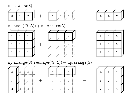
Broadcasting rules:
If the two arrays differ in their number of dimensions, the shape of the array with fewer dimensions is padded with ones on its leading (left) side.
If the shape of the two arrays does not match in any dimension, the array with shape equal to 1 in that dimension is stretched to match the other shape.
If in any dimension the sizes disagree and neither is equal to 1, an error is raised.
Some Broadcasting examples...
x = np.arange(10)
x ** 2
array([ 0, 1, 4, 9, 16, 25, 36, 49, 64, 81])
Y = x * x[:, np.newaxis]
Y
array([[ 0,  0,  0,  0,  0,  0,  0,  0,  0,  0],
       [ 0,  1,  2,  3,  4,  5,  6,  7,  8,  9],
       [ 0,  2,  4,  6,  8, 10, 12, 14, 16, 18],
       [ 0,  3,  6,  9, 12, 15, 18, 21, 24, 27],
       [ 0,  4,  8, 12, 16, 20, 24, 28, 32, 36],
       [ 0,  5, 10, 15, 20, 25, 30, 35, 40, 45],
       [ 0,  6, 12, 18, 24, 30, 36, 42, 48, 54],
       [ 0,  7, 14, 21, 28, 35, 42, 49, 56, 63],
       [ 0,  8, 16, 24, 32, 40, 48, 56, 64, 72],
       [ 0,  9, 18, 27, 36, 45, 54, 63, 72, 81]])
Y + 10 * x
array([[  0,  10,  20,  30,  40,  50,  60,  70,  80,  90],
       [  0,  11,  22,  33,  44,  55,  66,  77,  88,  99],
       [  0,  12,  24,  36,  48,  60,  72,  84,  96, 108],
       [  0,  13,  26,  39,  52,  65,  78,  91, 104, 117],
       [  0,  14,  28,  42,  56,  70,  84,  98, 112, 126],
       [  0,  15,  30,  45,  60,  75,  90, 105, 120, 135],
       [  0,  16,  32,  48,  64,  80,  96, 112, 128, 144],
       [  0,  17,  34,  51,  68,  85, 102, 119, 136, 153],
       [  0,  18,  36,  54,  72,  90, 108, 126, 144, 162],
       [  0,  19,  38,  57,  76,  95, 114, 133, 152, 171]])
Y + 10 * x[:, np.newaxis]
array([[  0,   0,   0,   0,   0,   0,   0,   0,   0,   0],
       [ 10,  11,  12,  13,  14,  15,  16,  17,  18,  19],
       [ 20,  22,  24,  26,  28,  30,  32,  34,  36,  38],
       [ 30,  33,  36,  39,  42,  45,  48,  51,  54,  57],
       [ 40,  44,  48,  52,  56,  60,  64,  68,  72,  76],
       [ 50,  55,  60,  65,  70,  75,  80,  85,  90,  95],
       [ 60,  66,  72,  78,  84,  90,  96, 102, 108, 114],
       [ 70,  77,  84,  91,  98, 105, 112, 119, 126, 133],
       [ 80,  88,  96, 104, 112, 120, 128, 136, 144, 152],
       [ 90,  99, 108, 117, 126, 135, 144, 153, 162, 171]])
Y = np.random.random((2, 3, 4))
x = 10 * np.arange(3)

Y + x[:, np.newaxis]
array([[[  0.16013996,   0.61070178,   0.70907938,   0.52638606],
        [ 10.74057435,  10.40082693,  10.48134161,  10.70561624],
        [ 20.45622939,  20.68181045,  20.40559978,  20.0304505 ]],

       [[  0.99607108,   0.93981662,   0.25316248,   0.41212159],
        [ 10.06903578,  10.41168541,  10.48591661,  10.24673383],
        [ 20.46827554,  20.32719887,  20.46975577,  20.39303078]]])
Quick Broadcasting Exercise
Now, assume you have $N$ points in $D$ dimensions, represented by an array of shape [N, D].
- Compute the mean of the distribution of points efficiently using the built-in
np.meanaggregate (that is, find theD-dimensional point which is the mean of the rest of the points) - Compute the mean of the distribution of points efficiently using the
np.addufunc. - Compute the standard error of the mean $\sigma_{mean} = \sigma N^{-1/2}$, where $\sigma$ is the standard-deviation, using the
np.stdaggregate. - Compute this again using the
np.addufunc. - Construct the matrix
M, the centered and normalized version of theXarray: $$ M_{ij} = (X_{ij} - \mu_j) / \sigma_j $$ This is one version of whitening the array.
X = np.random.random((1000, 5)) # 1000 points in 5 dimensions
# 1. Compute the mean of the 1000 points in X
# 2. Compute the standard deviation across the 1000 points
# 5. Compute the whitened version of the array
#    (Each row centered, then divided by standard deviation)
Strategy 4: Fancy Indexing and Masking
The last strategy we will cover is fancy indexing and masking.
For example, imagine you have an array of data where negative values indicate some kind of error.
x = np.array([1, 2, 3, -999, 2, 4, -999])
How might you clean this array, setting all negative values to, say, zero?
for i in range(len(x)):
    if x[i] < 0:
        x[i] = 0
x
array([1, 2, 3, 0, 2, 4, 0])
A faster way is to construct a boolean mask:
x = np.array([1, 2, 3, -999, 2, 4, -999])

mask = (x < 0)
mask
array([False, False, False, True, False, False, True], dtype=bool)
And the mask can be used directly to set the value you desire:
x[mask] = 0
x
array([1, 2, 3, 0, 2, 4, 0])
Typically this is done directly:
x = np.array([1, 2, 3, -999, 2, 4, -999])
x[x < 0] = 0
x
array([1, 2, 3, 0, 2, 4, 0])
Useful masking functions
x = np.random.random(5)
x
array([ 0.67649933, 0.96325803, 0.94898948, 0.44587652, 0.63444064])
x[x > 0.5] = np.nan
x
array([ nan, nan, nan, 0.44587652, nan])
x[np.isnan(x)] = np.inf
x
array([ inf, inf, inf, 0.44587652, inf])
np.nan == np.nan
False
x[np.isinf(x)] = 0
x
array([ 0. , 0. , 0. , 0.44587652, 0. ])
x = np.array([1, 0, -np.inf, np.inf, np.nan])
print("input   ", x)
print("x < 0   ", (x < 0))
print("x > 0   ", (x > 0))
print("isinf   ", np.isinf(x))
print("isnan   ", np.isnan(x))
print("isposinf", np.isposinf(x))
print("isneginf", np.isneginf(x))
input    [  1.   0. -inf  inf  nan]
x < 0    [False False  True False False]
x > 0    [ True False False  True False]
isinf    [False False  True  True False]
isnan    [False False False False  True]
isposinf [False False False  True False]
isneginf [False False  True False False]
-c:3: RuntimeWarning: invalid value encountered in less
-c:4: RuntimeWarning: invalid value encountered in greater
Boolean Operations on Masks
Use bitwise operators (and make sure to use parentheses!)
x = np.arange(16).reshape((4, 4))
x
array([[ 0,  1,  2,  3],
       [ 4,  5,  6,  7],
       [ 8,  9, 10, 11],
       [12, 13, 14, 15]])
x < 5
array([[ True,  True,  True,  True],
       [ True, False, False, False],
       [False, False, False, False],
       [False, False, False, False]], dtype=bool)
~(x < 5)
array([[False, False, False, False],
       [False,  True,  True,  True],
       [ True,  True,  True,  True],
       [ True,  True,  True,  True]], dtype=bool)
(x < 10) & (x % 2 == 0)
array([[ True, False,  True, False],
       [ True, False,  True, False],
       [ True, False, False, False],
       [False, False, False, False]], dtype=bool)
(x > 3) & (x < 8)
array([[False, False, False, False],
       [ True,  True,  True,  True],
       [False, False, False, False],
       [False, False, False, False]], dtype=bool)
Counting elements with a mask
Sum over a mask to find the number of True elements:
x = np.random.random(100)
print("array is length", len(x), "and has")
print((x > 0.5).sum(), "elements are greater than 0.5")
array is length 100 and has
61 elements are greater than 0.5
# clip is a useful function:
x = np.clip(x, 0.3, 0.6)

print(np.sum(x < 0.3))
print(np.sum(x > 0.6))
0
0
# works for 2D arrays as well
X = np.random.random((10, 10))
(X < 0.1).sum()
13
where function: Turning a mask into indices
x = np.random.random((3, 3))
x
array([[ 0.05999021,  0.03303966,  0.89629243],
       [ 0.87950144,  0.30331336,  0.17156985],
       [ 0.56147418,  0.2192196 ,  0.90690265]])
np.where(x < 0.3)
(array([0, 0, 1, 2]), array([0, 1, 2, 1]))
x[x < 0.3]
array([ 0.05999021, 0.03303966, 0.17156985, 0.2192196 ])
x[np.where(x < 0.3)]
array([ 0.05999021, 0.03303966, 0.17156985, 0.2192196 ])
When you index with the result of a where function, you are using what is called fancy indexing: indexing with tuples
Fancy Indexing (indexing with sequences)
X = np.arange(16).reshape((4, 4))
X
array([[ 0,  1,  2,  3],
       [ 4,  5,  6,  7],
       [ 8,  9, 10, 11],
       [12, 13, 14, 15]])
X[(0, 1), (1, 0)]
array([1, 4])
X[range(4), range(4)]
array([ 0, 5, 10, 15])
X.diagonal()
array([ 0, 5, 10, 15])
X.diagonal() = 100
  File "<ipython-input-101-3064a6b8dbd8>", line 1
    X.diagonal() = 100
                      ^
SyntaxError: can't assign to function call
X[range(4), range(4)] = 100
X
array([[100,   1,   2,   3],
       [  4, 100,   6,   7],
       [  8,   9, 100,  11],
       [ 12,  13,  14, 100]])
Randomizing the rows
X = np.arange(24).reshape((6, 4))
X
array([[ 0,  1,  2,  3],
       [ 4,  5,  6,  7],
       [ 8,  9, 10, 11],
       [12, 13, 14, 15],
       [16, 17, 18, 19],
       [20, 21, 22, 23]])
i = np.arange(6)
np.random.shuffle(i)
i
array([0, 1, 5, 4, 2, 3])
X[i] # X[i, :] is identical
array([[ 0,  1,  2,  3],
       [ 4,  5,  6,  7],
       [20, 21, 22, 23],
       [16, 17, 18, 19],
       [ 8,  9, 10, 11],
       [12, 13, 14, 15]])
Fancy indexing also works for multi-dimensional index arrays
i2 = i.reshape(3, 2)
X[i2]
array([[[ 0,  1,  2,  3],
        [ 4,  5,  6,  7]],

       [[20, 21, 22, 23],
        [16, 17, 18, 19]],

       [[ 8,  9, 10, 11],
        [12, 13, 14, 15]]])
X[i2].shape
(3, 2, 4)
Summary: Speeding up NumPy
It's all about moving loops into compiled code:
Use Numpy ufuncs to your advantage (eliminate loops!)
Use Numpy aggregates to your advantage (eliminate loops!)
Use Numpy broadcasting to your advantage (eliminate loops!)
Use Numpy slicing and masking to your advantage (eliminate loops!)
Use a tool like SWIG, cython or f2py to interface to compiled code.
Breakout: asteroid data
In the github repository, there is a file containing measurements of 5000 asteroid orbits, at notebooks/data/asteroids5000.csv.
These are compiled from a query at http://ssd.jpl.nasa.gov/sbdb_query.cgi
Part 1: loading and exploring the data
Use
np.genfromtxtto load the data from the file. This is likeloadtxt, but can handle missing data.- Remember to set the appropriate
delimiterkeyword.
- Remember to set the appropriate
genfromtxtsets all missing values tonp.nan. Use the operations we discussed here to answer these questions:- How many values are missing in this data?
- How many complete rows are there? i.e. how many objects have no missing values?
Create a new array containing only the rows with no missing values.
Compute the maximum, minimum, mean, and standard deviation of the values in each column.
Part 2: Plotting the data
Use the bash
headcommand to display the first line of the data file: this lists the names of the columns in the dataset. (remember that bash commands in the notebook are indicated by!, and thathead -ndisplays the firstnlines of a file)Invoke the
matplotlib inlinemagic to make figures appear inline in the notebookUse
plt.scatterto plot the semi-major axis versus the sine of the inclination angle (note that the inclination angle is listed in degrees -- you'll have to convert it to radians to compute the sine). What do you notice about the distribution? What do you think could explain this?Use
plt.scatterto plot a color-magnitude diagram of the asteroids (H vs B-V). You should see two distinct "families" of asteroids indicated in this plot. Over-plot a line that divides these.Repeat the orbital parameter plot from above, but plot the two "families" from #4 in different colors. Note that this magnitude is undefined for many of the asteroids. Do you see any correlation between color and orbit?
Compare what you found to plots in Parker et al. 2008. Note that we're not using the same data here, but we're looking at a similar collection of objects.