import numpy as np
import matplotlib.dates as mdates
import matplotlib.pyplot as plt
import matplotlib.patches as mpatches
from scipy.stats import norm
import time
from IPython.display import Image as ImageDisp
from sympy import Symbol, symbols, Matrix, sin, cos, latex, Plot
from sympy.interactive import printing
printing.init_printing()
%pylab inline --no-import-all
Populating the interactive namespace from numpy and matplotlib
Adaptive Extended Kalman Filter Implementation for Constant Turn Rate and Velocity (CTRV) Vehicle Model with Attitude Estimation in Python
for Testdataset generated by the 'DataGenerator.py'
Situation covered: You have an velocity sensor which measures the vehicle speed ($v$) in heading direction ($\psi$) and a yaw rate sensor ($\dot \psi$) which both have to fused with the position ($x$ & $y$) from a GPS sensor in loosely coupled way.
State Vector - Constant Turn Rate and Velocity Vehicle Model (CTRV) + Roll and Pitch Estimation
 $$x_k= \left[ \begin{matrix} x\\y\\ v \\ \psi\\\phi\\\Theta \end{matrix}\right] = \left[ \begin{matrix} \text{Position x (GNSS)}\\ \text{Position y (GNSS)}\\ \text{Speed (GNSS)} \\ \text{Heading (GNSS)} \\ \text{Pitch (IMU)} \\ \text{Roll (IMU)} \end{matrix}\right]$$
Here you can choose, wheather the following filter should work as a standard EKF or an adaptive one
adaptive = True
numstates=6 # States
dt    = 1.0/10.0 # Sample Rate of the Measurements is 50Hz
dtGPS = 1.0/10.0 # Sample Rate of GPS is 10Hz
All symbolic calculations are made with Sympy. Thanks!
vs, psis, dpsis, dts, xs, ys, axs, phis, dphis, thetas, dthetas, Lats, Lons = \
 symbols('v \psi \dot\psi T x y a_x \phi \dot\phi \Theta \dot\Theta Lat Lon')

As = Matrix([[xs+(vs/dpsis)*(sin(psis+dpsis*dts)-sin(psis))],
             [ys+(vs/dpsis)*(-cos(psis+dpsis*dts)+cos(psis))],
             [vs + axs*dts],
             [psis+dpsis*dts],
             [phis+dphis*dts],
             [thetas+dthetas*dts]])
state = Matrix([xs,ys,vs,psis,phis,thetas])
Dynamic Matrix
This formulas calculate how the state is evolving from one to the next time step
As
print latex(As)
\left[\begin{matrix}x + \frac{v}{\dot\psi} \left(- \sin{\left (\psi \right )} + \sin{\left (T \dot\psi + \psi \right )}\right)\\y + \frac{v}{\dot\psi} \left(\cos{\left (\psi \right )} - \cos{\left (T \dot\psi + \psi \right )}\right)\\T a_{x} + v\\T \dot\psi + \psi\\T \dot\phi + \phi\\T \dot\Theta + \Theta\end{matrix}\right]
Calculate the Jacobian of the Dynamic Matrix with respect to the state vector
state
As.jacobian(state)
It has to be computed on every filter step because it consists of state variables.
print latex(As.jacobian(state))
\left[\begin{matrix}1 & 0 & \frac{1}{\dot\psi} \left(- \sin{\left (\psi \right )} + \sin{\left (T \dot\psi + \psi \right )}\right) & \frac{v}{\dot\psi} \left(- \cos{\left (\psi \right )} + \cos{\left (T \dot\psi + \psi \right )}\right) & 0 & 0\\0 & 1 & \frac{1}{\dot\psi} \left(\cos{\left (\psi \right )} - \cos{\left (T \dot\psi + \psi \right )}\right) & \frac{v}{\dot\psi} \left(- \sin{\left (\psi \right )} + \sin{\left (T \dot\psi + \psi \right )}\right) & 0 & 0\\0 & 0 & 1 & 0 & 0 & 0\\0 & 0 & 0 & 1 & 0 & 0\\0 & 0 & 0 & 0 & 1 & 0\\0 & 0 & 0 & 0 & 0 & 1\end{matrix}\right]
It has to be computed on every filter step because it consists of state variables.
Real Measurements from Low Budget Hardware (IMU & GPS)
#path = './../RaspberryPi-CarPC/TinkerDataLogger/DataLogs/2014/'
#datafile = path+'2014-04-13-002-Data.csv'
datafile = 'testdata.csv'

xout, \
yout, \
speed, \
ax, \
course, \
yawrate, \
GNSSx, \
GNSSy, \
epe = np.loadtxt(datafile, delimiter=',', unpack=True)

val = len(xout)

ay = np.zeros(val)
az = np.zeros(val)-9.81
rollrate = np.zeros(val)
pitchrate = np.zeros(val)
roll = np.zeros(val)
pitch = np.zeros(val)
altitude = np.zeros(val)

print('Read \'%s\' successfully.' % datafile)
Read 'testdata.csv' successfully.
Control Input
control = Matrix([axs, dpsis, dphis, dthetas])
control
print latex(control)
\left[\begin{matrix}a_{x}\\\dot\psi\\\dot\phi\\\dot\Theta\end{matrix}\right]
Calculate the Jacobian of the Dynamic Matrix with Respect to the Control Input
JGs = As.jacobian(control)
JGs
print latex(JGs)
\left[\begin{matrix}0 & \frac{T v}{\dot\psi} \cos{\left (T \dot\psi + \psi \right )} - \frac{v}{\dot\psi^{2}} \left(- \sin{\left (\psi \right )} + \sin{\left (T \dot\psi + \psi \right )}\right) & 0 & 0\\0 & \frac{T v}{\dot\psi} \sin{\left (T \dot\psi + \psi \right )} - \frac{v}{\dot\psi^{2}} \left(\cos{\left (\psi \right )} - \cos{\left (T \dot\psi + \psi \right )}\right) & 0 & 0\\T & 0 & 0 & 0\\0 & T & 0 & 0\\0 & 0 & T & 0\\0 & 0 & 0 & T\end{matrix}\right]
Process Noise Covariance Matrix $Q$
Kelly, A. (1994). A 3D state space formulation of a navigation Kalman filter for autonomous vehicles, (May). Retrieved from http://oai.dtic.mil/oai/oai?verb=getRecord&metadataPrefix=html&identifier=ADA282853: "The state uncertainty model models the disturbances which excite the linear system. Conceptually, it estimates how bad things can get when the system is run open loop for a given period of time. The $Q$ matrix can be assumed diagonal, and its elements set to the predicted magnitude of the truncated terms in the constant velocity model. They can arise from:
- disturbances such as terrain following loads
- neglected control inputs such as sharp turns, braking or accelerating
- neglected derivatives in the dead reckoning model
- neglected states"
jerkmax = 300.0    # m/s3

pitchrateaccmax=  200.0 *np.pi/180.0 # rad/s2
rollrateaccmax =  200.0 *np.pi/180.0 # rad/s2
yawrateaccmax  =  80.0  *np.pi/180.0 # rad/s2
print('Sigma ax: %.2f m/s2' % (dt * jerkmax))
print('Sigma yaw: %.3f 1/s' % (dt * yawrateaccmax))
print('Sigma pitch: %.3f 1/s' % (dt * pitchrateaccmax))
print('Sigma roll: %.3f 1/s' % (dt * rollrateaccmax))
Sigma ax: 30.00 m/s2
Sigma yaw: 0.140 1/s
Sigma pitch: 0.349 1/s
Sigma roll: 0.349 1/s
Q = np.diagflat([[(dt * jerkmax)**2],            # acceleration
            [(dt * yawrateaccmax)**2],           # yawrate
            [(dt * pitchrateaccmax)**2],         # pitchrate
            [(dt * rollrateaccmax)**2]])         # rollrate
fig = plt.figure(figsize=(numstates, numstates))
im = plt.imshow(Q, interpolation="none", cmap=plt.get_cmap('binary'))
plt.title('Process Noise Covariance Matrix $Q$')
ylocs, ylabels = plt.yticks()
# set the locations of the yticks
plt.yticks(np.arange(6))
# set the locations and labels of the yticks
plt.yticks(np.arange(5), \
           ('$a_x$', '$\dot \psi$', '$\dot \phi$', '$\dot \Theta$'),\
           fontsize=22)

xlocs, xlabels = plt.xticks()
# set the locations of the yticks
plt.xticks(np.arange(6))
# set the locations and labels of the yticks
plt.xticks(np.arange(5), \
           ('$a_x$', '$\dot \psi$', '$\dot \phi$', '$\dot \Theta$'),\
           fontsize=22)

plt.xlim([-0.5,3.5])
plt.ylim([3.5, -0.5])

from mpl_toolkits.axes_grid1 import make_axes_locatable
divider = make_axes_locatable(plt.gca())
cax = divider.append_axes("right", "5%", pad="3%")
plt.colorbar(im, cax=cax)

plt.tight_layout()

Estimated Position Error
$EPE \sim \mathrm{HDOP} \cdot \mathrm{URA}(1 \sigma)$
plt.figure(figsize=(16,3))
plt.plot(epe, label='$EPE$ from GNSS modul', marker='*', markevery=50)
#plt.plot(speed)
plt.ylabel('$EPE$ in $(m)$')
plt.xlabel('Filterstep $k$')
plt.legend(loc='best')
#plt.savefig('Extended-Kalman-Filter-CTRV-Adaptive-R.png', dpi=72, transparent=True, bbox_inches='tight')
plt.savefig('Extended-Kalman-Filter-CTRV-EPE.eps', bbox_inches='tight')

Measurement Noise Covariance Matrix $R$ (Adaptive)
"In practical use, the uncertainty estimates take on the significance of relative weights of state estimates and measurements. So it is not so much important that uncertainty is absolutely correct as it is that it be relatively consistent across all models" - Kelly, A. (1994). A 3D state space formulation of a navigation Kalman filter for autonomous vehicles, (May). Retrieved from http://oai.dtic.mil/oai/oai?verb=getRecord&metadataPrefix=html&identifier=ADA282853
state
If adaptive=False, one have to determine the measurement noise covariances here:
R = np.diagflat([[(12.0)**2],      # x
            [(12.0)**2],           # y
            [(1.0)**2],  # v
            [(0.1)**2],  # heading
            [(0.5)**2],  # pitch
            [(0.5)**2]]) # roll
fig = plt.figure(figsize=(numstates, numstates))
im = plt.imshow(R, interpolation="none", cmap=plt.get_cmap('binary'))
plt.title('Measurement Noise Covariance Matrix $R$')
ylocs, ylabels = plt.yticks()
# set the locations of the yticks
plt.yticks(np.arange(7))
# set the locations and labels of the yticks
plt.yticks(np.arange(6), \
           ('$x$', '$y$', '$v$', '$\psi$', '$\phi$', '$\Theta$'),\
           fontsize=22)

xlocs, xlabels = plt.xticks()
# set the locations of the yticks
plt.xticks(np.arange(7))
# set the locations and labels of the yticks
plt.xticks(np.arange(6), \
           ('$x$', '$y$', '$v$', '$\psi$', '$\phi$', '$\Theta$'),\
           fontsize=22)

plt.xlim([-0.5,5.5])
plt.ylim([5.5, -0.5])

from mpl_toolkits.axes_grid1 import make_axes_locatable
divider = make_axes_locatable(plt.gca())
cax = divider.append_axes("right", "5%", pad="3%")
plt.colorbar(im, cax=cax)

plt.tight_layout()

Position
$R$ is just initialized here. In the Kalman Filter Step it will calculated dynamically with the $EPE$ (Estimated Position Error) from the GPS signal as well as depending on the $speed$, like proposed in [Wender, S. (2008). Multisensorsystem zur erweiterten Fahrzeugumfelderfassung. Retrieved from http://vts.uni-ulm.de/docs/2008/6605/vts_6605_9026.pdf P.108].
$\sigma_p^2 = c \cdot \sigma_\text{speed}^2 + \sigma_\text{EPE}^2$
with
$\sigma_\text{speed} = (v+\epsilon)^{-\xi}$
$\sigma_\text{EPE} = \zeta \cdot EPE$
epsilon = 0.1
xi      = 500.0
zeta    = 50.0

spspeed=xi/((speed/3.6)+epsilon)
spepe=zeta*epe
sp = (spspeed)**2 + (spepe)**2
plt.figure(figsize=(6,2))
plt.semilogy(spspeed**2, label='$\sigma_{x/y}$ from speed', marker='*', markevery=150)
plt.semilogy(spepe**2, label='$\sigma_{x/y}$ from EPE', marker='x', markevery=150)
plt.semilogy(sp, label='Res.', marker='o', markevery=150)
plt.ylabel('Values for $R$ Matrix')
plt.xlabel('Filterstep $k$')
#plt.legend(loc='best')
plt.legend(bbox_to_anchor=(0., 1.02, 1., .102), loc=3,
       ncol=3, mode="expand", borderaxespad=0.)
<matplotlib.legend.Legend at 0x127ca2290>

Attitude
Because the estimation of Roll and Pitch is only valid for quasistatic situations (which is not valid for a moving vehicle), the values for the measured rotations are dynamically chosen.
Uncertainty should be high when car is moving and very low, when the vehicle is standing still
$\sigma_\Theta=\sigma_\psi=\left[\rho+\gamma\cdot a\right]^2$
rho = 200.0
gamma=500.0

sroll = (rho + gamma*ay)**2
spitch= (rho + gamma*ax)**2
plt.figure(figsize=(6,2))
plt.semilogy(sroll, label='$\sigma_{\Theta}$', marker='o', markevery=150, alpha=0.8)
plt.semilogy(spitch, label='$\sigma_{\phi}$', marker='*', markevery=150, alpha=0.9)
plt.ylabel('Values for $R$ Matrix')
plt.xlabel('Filterstep $k$')
plt.legend(bbox_to_anchor=(0.0, 1.02, 1., .102), loc=3,
       ncol=2, mode="expand", borderaxespad=0.)
<matplotlib.legend.Legend at 0x12ec59490>

Measurement Function $h$
Matrix H is the Jacobian of the Measurement function h with respect to the state.
If GPS Measurement is available
hs = Matrix([[xs],[ys],[vs],[psis],[phis],[thetas]])
Hs=hs.jacobian(state)
Hs
Identity Matrix
I = np.eye(numstates)
print(I, I.shape)
(array([[ 1.,  0.,  0.,  0.,  0.,  0.],
       [ 0.,  1.,  0.,  0.,  0.,  0.],
       [ 0.,  0.,  1.,  0.,  0.,  0.],
       [ 0.,  0.,  0.,  1.,  0.,  0.],
       [ 0.,  0.,  0.,  0.,  1.,  0.],
       [ 0.,  0.,  0.,  0.,  0.,  1.]]), (6, 6))
Initial State
state
x = np.matrix([[0, 0, speed[0]/3.6, course[0], 0.0, 0.0]]).T
print(x, x.shape)

U=float(np.cos(x[3])*x[2])
V=float(np.sin(x[3])*x[2])

plt.quiver(x[0], x[1], U, V)
plt.scatter(float(x[0]), float(x[1]), s=100)
plt.title('Initial Location')
plt.axis('equal')
(matrix([[ 0.        ],
        [ 0.        ],
        [ 5.49555556],
        [ 0.        ],
        [ 0.        ],
        [ 0.        ]]), (6, 1))

Initial Uncertainty
Initialized with $0$ means you are pretty sure where the vehicle starts and in which direction it is heading. Initialized with high values means, that you trust the measurements first, to align the state vector $x$ with them.
P = 1e5*np.eye(numstates)
print(P.shape)

fig = plt.figure(figsize=(numstates, numstates))
im = plt.imshow(P, interpolation="none", cmap=plt.get_cmap('binary'))
plt.title('Covariance Matrix $P$')
ylocs, ylabels = plt.yticks()
# set the locations of the yticks
plt.yticks(np.arange(7))
# set the locations and labels of the yticks
plt.yticks(np.arange(6), \
           ('$x$', '$y$', '$v$', '$\psi$', '$\phi$', '$\Theta$'),\
           fontsize=22)

xlocs, xlabels = plt.xticks()
# set the locations of the yticks
plt.xticks(np.arange(7))
# set the locations and labels of the yticks
plt.xticks(np.arange(6), \
           ('$x$', '$y$', '$v$', '$\psi$', '$\phi$', '$\Theta$'),\
           fontsize=22)

plt.xlim([-0.5,5.5])
plt.ylim([5.5, -0.5])

from mpl_toolkits.axes_grid1 import make_axes_locatable
divider = make_axes_locatable(plt.gca())
cax = divider.append_axes("right", "5%", pad="3%")
plt.colorbar(im, cax=cax)

plt.tight_layout()
(6, 6)

Put everything together as a measurement vector
state
measurements = np.vstack((GNSSx, GNSSy, speed/3.6, course, roll, pitch))
# Lenth of the measurement
m = measurements.shape[1]
print(measurements.shape)
(6, 473)
# Preallocation for Plotting
x0 = []
x1 = []
x2 = []
x3 = []
x4 = []
x5 = []
x6 = []
x7 = []
x8 = []
Zx = []
Zy = []
P0 = []
P1 = []
P2 = []
P3 = []
P4 = []
P5 = []
P6 = []
P7 = []
P8 = []
K0 = []
K1 = []
K2 = []
K3 = []
K4 = []
K5 = []
dstate=[]
starttime = time.time()
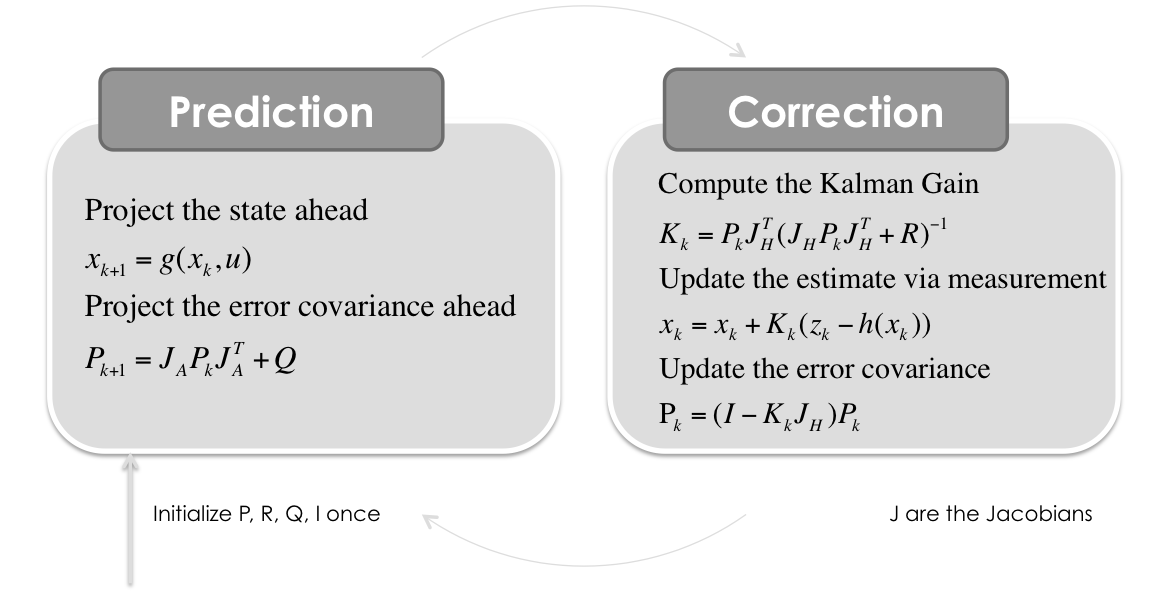
Extended Kalman Filter Step
for filterstep in range(m):

    axc = -ax[filterstep]
    yawc = yawrate[filterstep]
    pitc = pitchrate[filterstep]/180.0*np.pi
    rolc = rollrate[filterstep]/180.0*np.pi

    # Time Update (Prediction)
    # ========================
    # Project the state ahead
    # see "Dynamic Matrix"
    if yawc==0.0: # Driving straight
        x[0] = x[0] + x[2]*dt * np.cos(x[3])
        x[1] = x[1] + x[2]*dt * np.sin(x[3])
        x[2] = x[2] + axc*dt
        x[3] = x[3]
        x[4] = x[4] + pitc*dt
        x[5] = x[5] + rolc*dt
        yawc = 0.00000001 # to avoid numerical issues in Jacobians
        dstate.append(0)
    else: # otherwise
        x[0] = x[0] + (x[2]/yawc) * (np.sin(yawc*dt+x[3]) - np.sin(x[3]))
        x[1] = x[1] + (x[2]/yawc) * (-np.cos(yawc*dt+x[3])+ np.cos(x[3]))
        x[2] = x[2] + axc*dt
        x[3] = (x[3] + yawc*dt + np.pi) % (2.0*np.pi) - np.pi
        x[4] = x[4] + pitc*dt
        x[5] = x[5] + rolc*dt
        dstate.append(1)

    # Calculate the Jacobian of the Dynamic Matrix A
    # see "Calculate the Jacobian of the Dynamic Matrix with respect to the state vector"
    a13 = float((1.0/yawc) * (np.sin(yawc*dt+x[3]) - np.sin(x[3])))
    a14 = float((x[2]/yawc)* (np.cos(yawc*dt+x[3]) - np.cos(x[3])))
    a23 = float((1.0/yawc) * (-np.cos(yawc*dt+x[3]) + np.cos(x[3])))
    a24 = float(x[2]/yawc) * (np.sin(yawc*dt+x[3]) - np.sin(x[3]))
    JA = np.matrix([[1.0, 0.0, a13, a14, 0.0, 0.0],
                  [0.0, 1.0, a23, a24, 0.0, 0.0],
                  [0.0, 0.0, 1.0, 0.0, 0.0, 0.0],
                  [0.0, 0.0, 0.0, 1.0, 0.0, 0.0],
                  [0.0, 0.0, 0.0, 0.0, 1.0, 0.0],
                  [0.0, 0.0, 0.0, 0.0, 0.0, 1.0]])

    # Calculate the Jacobian of the Control Input G
    # see "Calculate the Jacobian of the Dynamic Matrix with Respect to the Control"
    g12 = float((dt*x[2]/yawc)*np.cos(yawc*dt+x[3]) - x[2]/yawc**2*(np.sin(yawc*dt+x[3])-np.sin(x[3])))
    g22 = float((dt*x[2]/yawc)*np.sin(yawc*dt+x[3]) - x[2]/yawc**2*(-np.cos(yawc*dt+x[3])+np.cos(x[3])))
    JG = np.matrix([[0.0, g12, 0.0, 0.0],
                    [0.0, g22, 0.0, 0.0],
                    [dt, 0.0, 0.0, 0.0],
                    [0.0, dt, 0.0, 0.0],
                    [0.0, 0.0, dt, 0.0],
                    [0.0, 0.0, 0.0, dt]])

    # Project the error covariance ahead
    P = JA*P*JA.T + JG*Q*JG.T


    # Measurement Update (Correction)
    # ===============================
    hx = np.matrix([[float(x[0])],
                    [float(x[1])],
                    [float(x[2])],
                    [float(x[3])],
                    [float(x[4])],
                    [float(x[5])]])
    # Because GPS is sampled with 10Hz and the other Measurements, as well as
    # the filter are sampled with 50Hz, one have to wait for correction until
    # there is a new GPS Measurement

    # Calculate the Jacobian of the Measurement Function
    # see "Measurement Matrix H"
    JH = np.matrix([[1.0, 0.0, 0.0, 0.0, 0.0, 0.0],
                    [0.0, 1.0, 0.0, 0.0, 0.0, 0.0],
                    [0.0, 0.0, 1.0, 0.0, 0.0, 0.0],
                    [0.0, 0.0, 0.0, 1.0, 0.0, 0.0],
                    [0.0, 0.0, 0.0, 0.0, 1.0, 0.0],
                    [0.0, 0.0, 0.0, 0.0, 0.0, 1.0]])

    if adaptive:
        # Adaptive R
        R[0,0] = sp[filterstep]       # x
        R[1,1] = sp[filterstep]       # y
        R[2,2] = spspeed[filterstep]  # v
        R[3,3] = spspeed[filterstep]  # course
        R[4,4] = spitch[filterstep]   # pitch
        R[5,5] = sroll[filterstep]    # roll


    S = JH*P*JH.T + R
    K = (P*JH.T) * np.linalg.inv(S)

    # Update the estimate via
    z = measurements[:,filterstep].reshape(JH.shape[0],1)
    y = z - (hx)                         # Innovation or Residual
    x = x + (K*y)

    # Update the error covariance
    P = (I - (K*JH))*P


    # Save states for Plotting
    x0.append(float(x[0]))
    x1.append(float(x[1]))
    x2.append(float(x[2]))
    x3.append(float(x[3]))
    x4.append(float(x[4]))
    x5.append(float(x[5]))

    P0.append(float(P[0,0]))
    P1.append(float(P[1,1]))
    P2.append(float(P[2,2]))
    P3.append(float(P[3,3]))
    P4.append(float(P[4,4]))
    P5.append(float(P[5,5]))

    #Zx.append(float(z[0]))
    #Zy.append(float(z[1]))

    K0.append(float(K[0,0]))
    K1.append(float(K[1,0]))
    K2.append(float(K[2,0]))
    K3.append(float(K[3,0]))
    K4.append(float(K[4,0]))
print('One Filterstep took %.4fs (average) on MacBook Pro 2.5GHz Intel i5' % ((time.time() - starttime)/m))
One Filterstep took 0.0049s (average) on MacBook Pro 2.5GHz Intel i5
Plots
%pylab inline --no-import-all
Populating the interactive namespace from numpy and matplotlib
Uncertainties of Matrix $P$
fig = plt.figure(figsize=(16,9))
plt.semilogy(range(m),P0, label='$x$')
plt.step(range(m),P1, label='$y$')
plt.step(range(m),P2, label='$v$')
plt.step(range(m),P3, label='$\psi$')
plt.step(range(m),P4, label='$\phi$')
plt.step(range(m),P5, label='$\Theta$')

plt.xlabel('Filter Step [k]')
plt.ylabel('')

plt.title('Uncertainty (Elements from Matrix $P$)')
#plt.legend(loc='best',prop={'size':22})
plt.legend(bbox_to_anchor=(0., 0.91, 1., .06), loc=3,
       ncol=9, mode="expand", borderaxespad=0.,prop={'size':22})
<matplotlib.legend.Legend at 0x12bee09d0>

fig = plt.figure(figsize=(numstates, numstates))
im = plt.imshow(P, interpolation="none", cmap=plt.get_cmap('binary'))
plt.title('Covariance Matrix $P$')
ylocs, ylabels = plt.yticks()
# set the locations of the yticks
plt.yticks(np.arange(7))
# set the locations and labels of the yticks
plt.yticks(np.arange(6), \
           ('$x$', '$y$', '$v$', '$\psi$', '$\phi$', '$\Theta$'),\
           fontsize=22)

xlocs, xlabels = plt.xticks()
# set the locations of the yticks
plt.xticks(np.arange(7))
# set the locations and labels of the yticks
plt.xticks(np.arange(6), \
           ('$x$', '$y$', '$v$', '$\psi$', '$\phi$', '$\Theta$'),\
           fontsize=22)

plt.xlim([-0.5,5.5])
plt.ylim([5.5, -0.5])

from mpl_toolkits.axes_grid1 import make_axes_locatable
divider = make_axes_locatable(plt.gca())
cax = divider.append_axes("right", "5%", pad="3%")
plt.colorbar(im, cax=cax)

plt.tight_layout()

Kalman Gains in $K$
fig = plt.figure(figsize=(16,9))
plt.step(range(len(measurements[0])),K0, label='$x$')
plt.step(range(len(measurements[0])),K1, label='$y$')
plt.step(range(len(measurements[0])),K2, label='$\psi$')
plt.step(range(len(measurements[0])),K3, label='$v$')
plt.step(range(len(measurements[0])),K4, label='$\dot \psi$')

plt.xlabel('Filter Step [k]')
plt.ylabel('')
plt.title('Kalman Gain (the lower, the more the measurement fullfill the prediction)')
#plt.legend(prop={'size':18})
plt.legend(bbox_to_anchor=(0., 0., 1., .102), loc=3,
       ncol=5, mode="expand", borderaxespad=0.,prop={'size':22})
plt.ylim([-0.4,0.4])

State Vector
state
fig = plt.figure(figsize=(8,numstates+2))

# Speed
plt.subplot(411)
plt.step(range(len(measurements[0])),np.multiply(x2,3.6), label='$v$', marker='*', markevery=140)
plt.step(range(len(measurements[0])),speed, label='$v$ (GNSS)', marker='o', markevery=150, alpha=0.6)
plt.ylabel('Speed $km/h$')
#plt.yticks(np.arange(-180, 181, 45))
#plt.ylim([0,60])
plt.legend(bbox_to_anchor=(0.25, 0.75, 0.35, .06), loc=3,
       ncol=2, mode="expand", borderaxespad=0.)

# Course
plt.subplot(412)
plt.step(range(len(measurements[0])),np.multiply(x3,180.0/np.pi), label='$\psi$', marker='*', markevery=140)
plt.step(range(len(measurements[0])),(180.0/np.pi*course+180.0)%(360.0)-180.0, label='$\psi$ (GNSS)', marker='o', markevery=150, alpha=0.6)
plt.ylabel('Course $^\circ$')
plt.yticks(np.arange(-180, 181, 45))
plt.ylim([-200,200])
plt.legend(bbox_to_anchor=(0.65, 0.0, 0.35, .06), loc=3,
       ncol=2, mode="expand", borderaxespad=0.)
#plt.title('State Estimates $x_k$')

# Pitch
plt.subplot(413)
plt.step(range(len(measurements[0])),np.multiply(x4,180.0/np.pi), label='$\phi$', marker='*', markevery=140)
plt.ylabel('Pitch $^\circ$')
plt.ylim([-10.0, 10.0])
plt.legend(loc='best',prop={'size':12})

# Roll
plt.subplot(414)
plt.step(range(len(measurements[0])),np.multiply(x5,180.0/np.pi), label='$\Theta$', marker='*', markevery=140)
plt.ylabel('Roll $^\circ$')
plt.ylim([-10.0, 10.0])
plt.legend(loc='best',prop={'size':12})

plt.xlabel('Filter Step $k$')
<matplotlib.text.Text at 0x12f6fe6d0>

#%pylab --no-import-all
Position X/Y
fig = plt.figure(figsize=(8,3))

# EKF State
#qscale= 0.5*np.divide(x3,np.max(x3))+0.1
#plt.quiver(x0,x1,np.cos(x2), np.sin(x2), color='#94C600', units='xy', width=0.01, scale=qscale)
plt.plot(x0,x1, color='k', label='EKF Position', linewidth=5)

# Ground Truth
plt.plot(xout, yout, label='Ground Truth')

# Measurements
if adaptive:
    plt.scatter(GNSSx,GNSSy, s=50, label='GNSS Measurements', c=sp, cmap='winter',norm=matplotlib.colors.LogNorm())
    cbar=plt.colorbar()
    cbar.ax.set_ylabel(u'$\sigma^2_x$ and $\sigma^2_y$', rotation=270)
    #cbar.ax.set_xlabel(u'm')
    #plt.title('Performance of adaptive EKF with values of measurement uncertainty $R$ (color)')
else:
    plt.scatter(GNSSx,GNSSy, s=20, label='GPS Measurements', c='g')
    #plt.title('Performance of EKF with static $R$')


plt.xlabel('X [m]')
plt.ylabel('Y [m]')

plt.axis('equal')
plt.xlim([-10, np.max(xout)+10])
plt.ylim(-80, 40)

# Annotations
bbox_props = dict(boxstyle="square,pad=0.9", fc="k", ec="w", lw=2)
t = plt.text(160, -30, "B", ha="left", va="center", rotation=0,
            size=16, color='grey',
            bbox=bbox_props)

plt.annotate('stop', xy=(30, -20), xytext=(60, -50), fontsize=16,
            arrowprops=dict(facecolor='k', shrink=0.05), ha='center',
            )

plt.legend(loc='lower right')

plt.tight_layout()

#plt.show()
if adaptive:
    plt.savefig('Extended-Kalman-Filter-CTRV-Position-Testdata.eps', bbox_inches='tight')
else:
    plt.savefig('Extended-Kalman-Filter-CTRV-Position-Testdata-NonAdaptive.eps', bbox_inches='tight')

Calculate the Error
CTEy = (x1 - yout)
CTEx = (x0 - xout)

sCTEy = np.sum(CTEy**2)
sCTEx = np.sum(CTEx**2)
fig = plt.figure(figsize=(8,3))
plt.plot(xout, CTEx, label='$CTE_x$, $\Sigma(CTE_x^2)$=%.0f$m^2$' % sCTEx)
plt.plot(xout, CTEy, label='$CTE_y$, $\Sigma(CTE_y^2)$=%.0f$m^2$' % sCTEy)
plt.xlabel('X [m]')
plt.ylabel('CTE [m]')
if adaptive:
    plt.title(r'$CTE$ of Position Estimation for $\epsilon=$ %.2f, $\xi=$ %.2f, $\zeta=$ %.2f' % (epsilon, xi, zeta))
else:
    plt.title('$CTE$ of Position Estimation with static $R$')
plt.legend(loc='best')
plt.axis('equal')
plt.xlim([-10, np.max(xout)+10])
plt.ylim(-80, 40)

# Annotations
bbox_props = dict(boxstyle="square,pad=0.9", fc="k", ec="w", lw=2)
t = plt.text(160, -30, "B", ha="left", va="center", rotation=0,
            size=16, color='grey',
            bbox=bbox_props)

plt.annotate('stop', xy=(30, -20), xytext=(60, -50), fontsize=16,
            arrowprops=dict(facecolor='k', shrink=0.05), ha='center',
            )

plt.legend(loc='lower right')

plt.tight_layout()

if adaptive:
    plt.savefig('Extended-Kalman-Filter-CTRV-CTE-Testdata.eps', bbox_inches='tight')
else:
    plt.savefig('Extended-Kalman-Filter-CTRV-CTE-Testdata-NonAdaptive.eps', bbox_inches='tight')

Dictionaries of Measurements
CTE = {}
CTE['Adaptive'] = {}
CTE['Non-Adaptive']={}

CTE['Non-Adaptive']['X'] = (928.0, 1404.0, 1312.0, 905.0, 1711.0)
CTE['Non-Adaptive']['Y'] = (2442.0, 2048.0, 2586.0, 2554.0, 1585.0)

CTE['Adaptive']['X'] = (221.0, 253.0, 219.0, 272.0, 212.0)
CTE['Adaptive']['Y'] = (404.0, 344.0, 430.0, 390.0, 409.0)
Normalize it
CTE['Adaptive']['X'] = np.divide(CTE['Adaptive']['X'], np.median(CTE['Non-Adaptive']['X']))
CTE['Adaptive']['Y'] = np.divide(CTE['Adaptive']['Y'], np.median(CTE['Non-Adaptive']['Y']))
CTE['Non-Adaptive']['X'] = np.divide(CTE['Non-Adaptive']['X'], np.median(CTE['Non-Adaptive']['X']))
CTE['Non-Adaptive']['Y'] = np.divide(CTE['Non-Adaptive']['Y'], np.median(CTE['Non-Adaptive']['Y']))
fig, axes = plt.subplots(ncols=2, sharey=True)

for ax, name in zip(axes, ['Non-Adaptive', 'Adaptive']):
    ax.boxplot([CTE[name][item] for item in ['X', 'Y']])
    ax.set(xticklabels=['X', 'Y'], xlabel=name)
    ax.set(ylabel='normalized $\Sigma$ CTE $(-)$')
    ax.margins(0.05) # Optional

plt.savefig('CTE-Adaptive-NonAdaptive-Boxplot.eps', bbox_inches='tight')

print('CTE reduced in X: %.0f%%' % (100.0-100.0*np.mean(CTE['Adaptive']['X']) / np.mean(CTE['Non-Adaptive']['X'])))
print('CTE reduced in Y: %.0f%%' % (100.0-100.0*np.mean(CTE['Adaptive']['Y']) / np.mean(CTE['Non-Adaptive']['Y'])))
CTE reduced in X: 81%
CTE reduced in Y: 82%
Works just fine!