Rolling Imbalance
MCHE 513: Intermediate Dynamics
Dr. Joshua Vaughan
joshua.vaughan@louisiana.edu
http://www.ucs.louisiana.edu/~jev9637/
The notebook will form the equations of motion for an unbalanced rolling cylinder, with eccentricity $\epsilon$ and radius $R$. There is enough friction such that pure rolling (no slip) is maintained. The system is sketched in Figure 1.
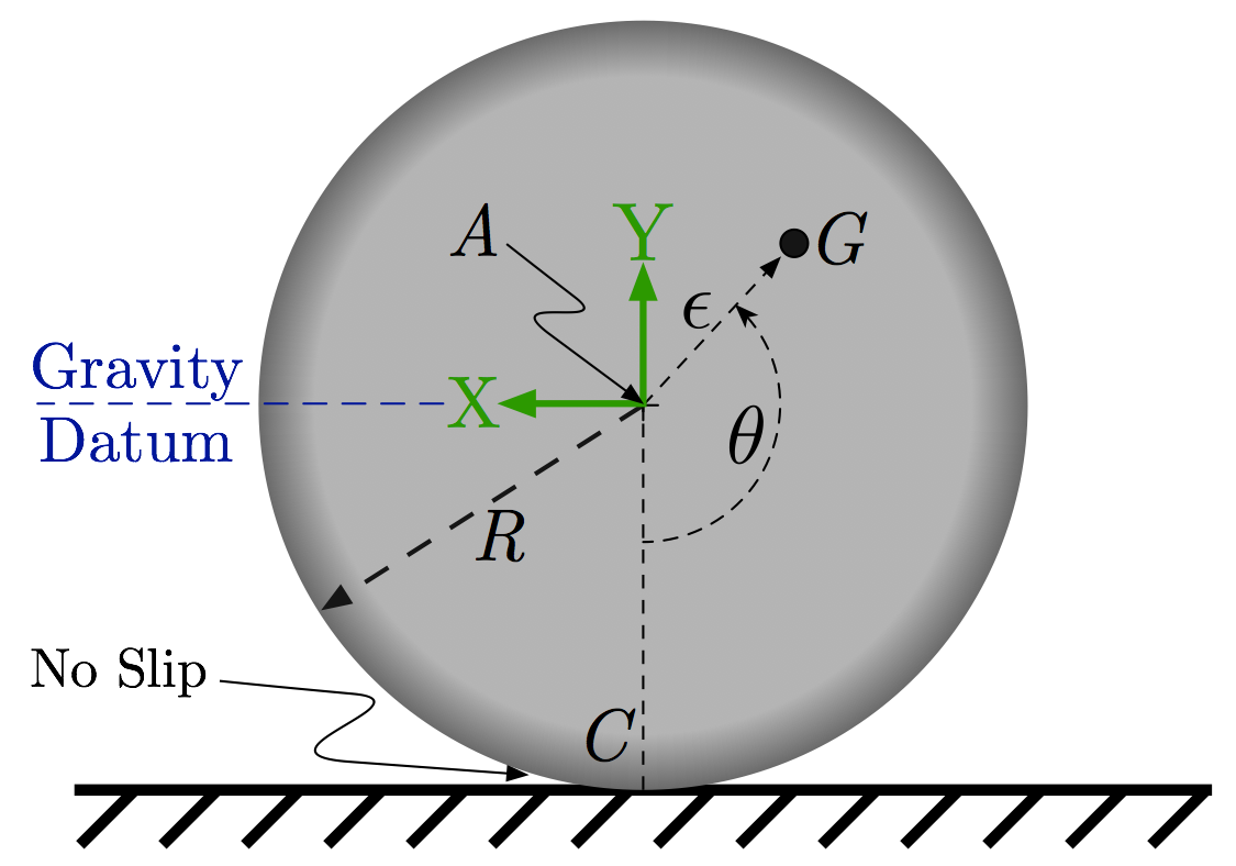
Figure 1: Rolling Cylinder with Imbalance
# Import the SymPy Module
import sympy

# Import the necessary sub-modules and methods for dynamics
from sympy.physics.mechanics import dynamicsymbols, inertia
from sympy.physics.mechanics import LagrangesMethod, Lagrangian
from sympy.physics.mechanics import Particle, Point, ReferenceFrame, RigidBody

# initiate better printing of SymPy results
sympy.init_printing()
# Define the generalized coordinates - just 1DOF here
theta = dynamicsymbols('theta')
theta_dot = dynamicsymbols('theta', 1)

# Define the other symbols needed
R, e, m, g, Izz, t = sympy.symbols('R epsilon m g I_{zz} t')
# Define the Newtonian reference frame
N = ReferenceFrame('N')

# Define a body-fixed frame along the pendulum, with y aligned from m to the pin
P = N.orientnew('P', 'Axis', [-theta, N.z])

# Define the point at the center of the cylinder and set its velocity
A = Point('A')
A.set_vel(N, R * theta_dot * N.x) # Pure rolling
# Locate the center of mass relative to the cylinder center
G = A.locatenew('G', -e * (sympy.sin(theta) * N.x + sympy.cos(theta) * N.y))

# Define its velocity, working from the velocity of point A - needed for kinetic energy calculation
G.v2pt_theory(A, N, P)
# Create the inertia diadic for the cylinder.
# Since the system is planar, set Ixx and Iyy to zero for simplicity
Ic = inertia(P, 0, 0, Izz)

# Define the cylinder as a rigid body
cylinder = RigidBody('cylinder', G, P, m, (Ic, G))

# Define the potential energy of the cyliner - just gravity here
cylinder.potential_energy =-m * g * e * sympy.cos(theta)
# Form the Lagrangian, then simplify and print
L = Lagrangian(N, cylinder)
L.simplify()
# create an instance of the LagrangesMethod class
LM = LagrangesMethod(L, [theta])

# Form the equations of motion, then simplify and print
eq_of_motion = LM.form_lagranges_equations()
sympy.collect(sympy.simplify(eq_of_motion)[0], theta)
Simulation
We can pass these equations of motion to numerical solver for simluation. To do so, we need to import NumPy and the SciPy ode solver, ode. We'll also import matplotlib to enable plotting of the results.
For a system as simple as this one, we could easily set up the necessary components for the numerical simulation manually. However, here we will automate as much as possible. Following a similar procedure on more complicated systems would be necessary.
# import NumPy with namespace np
import numpy as np

# import the ode ODE solver
from scipy.integrate import ode

# import the plotting functions from matplotlib
import matplotlib.pyplot as plt

# set up the notebook to display the plots inline
%matplotlib inline
# Make the call to set up in state-space-ish form q_dot = f(q, t)
lrhs = LM.rhs()

# Simplify the results
lrhs.simplify()

# Output the result
lrhs
# Define the states and state vector
w1, w2 = sympy.symbols('w1 w2', cls=sympy.Function)
w = [w1(t), w2(t)]

# Set up the state definitions and parameter substitution
sub_params = {theta: w1(t),
              theta_dot: w2(t),
              g : 9.81,
              e : 0.5,
              R : 1.0,
              m : 10.0,
              Izz : 0.5 * (0.9 * m) * R**2 + (0.1 * m) * e**2}

# Create a function from the equations of motion
# Here, we substitude the states and parameters as appropriate prior to the lamdification
eq_of_motion = sympy.lambdify((t, w),
                              lrhs.subs(sub_params))
# Set up the initial conditions for the solver
theta_init = 225 * np.pi/180     # Initial angle
theta_dot_init = 0           # Initial angular velocity

# Pack the initial conditions into an array
x0 = [theta_init, theta_dot_init]

# Create the time samples for the output of the ODE solver
sim_time = np.linspace(0.0, 10.0, 1001) # 0-10s with 1001 points in between
# Set up the initial point for the ode solver
r = ode(eq_of_motion).set_initial_value(x0, sim_time[0])

# define the sample time
dt = sim_time[1] - sim_time[0]

# pre-populate the response array with zeros
response = np.zeros((len(sim_time), len(x0)))

# Set the initial index to 0
index = 0

# Now, numerically integrate the ODE while:
#   1. the last step was successful
#   2. the current time is less than the desired simluation end time
while r.successful() and r.t < sim_time[-1]:
    response[index, :] = r.y
    r.integrate(r.t + dt)
    index += 1
# Set the plot size - 3x2 aspect ratio is best
fig = plt.figure(figsize=(6, 4))
ax = plt.gca()
plt.subplots_adjust(bottom=0.17, left=0.17, top=0.96, right=0.96)

# Change the axis units to serif
plt.setp(ax.get_ymajorticklabels(), family='serif', fontsize=18)
plt.setp(ax.get_xmajorticklabels(), family='serif', fontsize=18)

# Remove top and right axes border
ax.spines['right'].set_color('none')
ax.spines['top'].set_color('none')

# Only show axes ticks on the bottom and left axes
ax.xaxis.set_ticks_position('bottom')
ax.yaxis.set_ticks_position('left')

# Turn on the plot grid and set appropriate linestyle and color
ax.grid(True,linestyle=':', color='0.75')
ax.set_axisbelow(True)

# Define the X and Y axis labels
plt.xlabel('Time (s)', family='serif', fontsize=22, weight='bold', labelpad=5)
plt.ylabel('Angle (deg)', family='serif', fontsize=22, weight='bold', labelpad=10)

# Plot the data
plt.plot(sim_time, response[:, 0] * 180/np.pi, linewidth=2, linestyle='-', label = '$\theta$')

# uncomment below and set limits if needed
# plt.xlim(0, 5)
# plt.ylim(-1, 1)

# Create the legend, then fix the fontsize
# leg = plt.legend(loc='upper right', ncol = 1, fancybox=True)
# ltext  = leg.get_texts()
# plt.setp(ltext, family='serif', fontsize=20)

# Adjust the page layout filling the page using the new tight_layout command
plt.tight_layout(pad=0.5)

# Uncomment to save the figure as a high-res pdf in the current folder
# It's saved at the original 6x4 size
# plt.savefig('Simple_Pendulum_Response.pdf')

fig.set_size_inches(9, 6) # Resize the figure for better display in the notebook

Let's plot the planar position of the center of mass.
x = 2 * 1.0 * np.pi * response[:,0] - 0.1 * np.sin(response[:,0])
y = -0.1 * np.cos(response[:,0])
# Set the plot size - 3x2 aspect ratio is best
fig = plt.figure(figsize=(6, 4))
ax = plt.gca()
plt.subplots_adjust(bottom=0.17, left=0.17, top=0.96, right=0.96)

# Change the axis units to serif
plt.setp(ax.get_ymajorticklabels(), family='serif', fontsize=18)
plt.setp(ax.get_xmajorticklabels(), family='serif', fontsize=18)

# Remove top and right axes border
ax.spines['right'].set_color('none')
ax.spines['top'].set_color('none')

# Only show axes ticks on the bottom and left axes
ax.xaxis.set_ticks_position('bottom')
ax.yaxis.set_ticks_position('left')

# Turn on the plot grid and set appropriate linestyle and color
ax.grid(True,linestyle=':', color='0.75')
ax.set_axisbelow(True)

# Define the X and Y axis labels
plt.xlabel('Horizontal Position (m)', family='serif', fontsize=22, weight='bold', labelpad=5)
plt.ylabel('Vertical Position (m)', family='serif', fontsize=22, weight='bold', labelpad=10)

# Plot the data
plt.plot(x, y, linewidth=2, linestyle='-')

# uncomment below and set limits if needed
# plt.xlim(-1, 1)
# plt.ylim(1.25*np.min(y), 0.01)

# Adjust the page layout filling the page using the new tight_layout command
plt.tight_layout(pad=0.5)

# Uncomment to save the figure as a high-res pdf in the current folder
# It's saved at the original 6x4 size
# plt.savefig('Spring_Pendulum_Response_Planar.pdf')

fig.set_size_inches(9, 6) # Resize the figure for better display in the notebook

Licenses
Code is licensed under a 3-clause BSD style license. See the licenses/LICENSE.md file.
Other content is provided under a Creative Commons Attribution-NonCommercial 4.0 International License, CC-BY-NC 4.0.
# This cell will just improve the styling of the notebook
# You can ignore it, if you are okay with the default sytling
from IPython.core.display import HTML
import urllib.request
response = urllib.request.urlopen("https://cl.ly/1B1y452Z1d35")
HTML(response.read().decode("utf-8"))