
NumPy arrays: Creation and handling
Computer tools for Astronomers
This first part is an enhanced version of the slide about fundamental array handling in Numpy/SciPy.
Basically, all I have done here is to add some plots that visualize the arrays with colors, because it makes it clearer what happens when we perform the different operations .For thispurpose, I am introducing the function imshow() from Matplotlib. We shall look more at plotting later; for now it is enough to know that imshow() can translate the value of each array element into a color, which can make it quite a bit easier to see whatis going on in the array than just looking at a bunch of numbers.
Please note: I am using the notebook interface to write this, since it is great for making demos of all the feature. However, I recommend that you try the code below in the terminal or QtConsole interface, as these have some features that this doesn't. For example, the plots will show up in an interactive window that allow, panning zooming, etc., unlike this interface that produces static raster images of the plots.
import scipy as sp
import matplotlib.pyplot as plt
from scipy import random as ra   # Purely laziness
# Only do this if you are working in the Notebook interface:
%matplotlib inline
Array construction
The simplest way to define an array is by feeding it a list of numbers.
a = sp.array([1., 2., 3.])
print a
If you want a 2D array, feed it a list of lists of numbers:
a = sp.array([[1., 2., 3.],
              [4., 5., 6.],
              [7., 8., 9.]])
print a
NB! In the above, the line breaks are only there to look good. We could just as well have written:
a = sp.array([[1., 2., 3.], [4., 5., 6.], [7., 8., 9.]])
Now I have been reassigning values to the variable name 'a' a few times. Let's keep it the next time:
a = sp.zeros((8, 8)); print a
What we wrote here was "create an array of $8 \times 8$ elements and set them all to zero".
There's another convenience function called ones(), which can also be called with a tuple of numbers:
b = sp.ones((8, 8))
print b
Besides, there are also the convenience functions zeros_like() and ones_like() that take another array as the input and returns an array of zeros resp. ones of the same size as the input array:
b = sp.ones_like(a)
print(b)
An array can be reshaped to any shape you want, as long as it has the correct number of elements:
b = sp.ones_like(a).reshape((4, 16))
print b
print(b.transpose())   # Or b.T = easier to write but less explicit.
b = b.reshape((8, 8))  # Just to get the good ol' `b` array back.
There are a number of different random number generating functions, the simplest of which is scipy.random.random().
Since in the imports section we have already abbreviated scipy.random to ra, we can write this as:
c = ra.random(b.shape)
Remember, you can always get help for a function by writing e.g. ra.random? in your IPython console.
Printing an array of random floating point numbers between zero and one doesn't show much, so we will visualize the array with a plotting function instead. Try running the below commands a few times to convince yourself that it is in fact a pretty well randomized set you get:
# This cell should be ignored or deleted...
plt.colormaps?
plt.set_cmap('hot')
c = ra.random(b.shape) * .5
plt.matshow(c)
plt.colorbar()
# plt.show()  # Remember to write this when calling it from the terminal
Another convenience function gives you the Identity matrix, usually called $I$. Since I is a bad name for a function, they called it something very similar yet not the same:
d = sp.eye(b.shape[0]); print(d)
plt.matshow(d); plt.colorbar()
#b.shape    # Arribute
#b.max()    # Method
Array vs. matrix
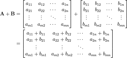
Unlike e.g. Matlab$^®$, NumPy doesn't perform matrix operations by default, but only when you specifically ask about it. If we use the arrays c and d as examples, the difference is quite clear. Taking the sum of the two is the same in both languages, as the matrix sum is just defined as the element-wise sum like it is explained in wikipedia:
In our case, the sum of c and d, hardly surprising, becomes:
plt.matshow(c + d, interpolation='nearest'); plt.colorbar()
However, in in NumPy our array is *not treated as a matrix unless we explicitly do this*.
Here's the difference (by the way, compare the diagonals):
array_product = c * d           # Element-wise product
matrix_product = sp.dot(d, c)   # Matrix product

# And now some plotting magic:
plt.subplot(121)
plt.imshow(array_product, interpolation='nearest')
plt.title('Element wise `Array` product \n default in NumPy')
plt.subplot(122)
plt.imshow(matrix_product, interpolation='nearest')
plt.title('`Matrix` product \n default in Matlab/Octave')
# plt.show()
Let's call c and d interpreted as matrices $C$ and $D$, respectively.
Since $D$ is the identity matrix, it should come as no surprise that $D C = C$.
Reshaping
As mentioned, arrays are easily reshaped, as long as you don't mess up the total number of elements:
e = sp.arange(64).reshape(1, -1)   # '-1' here means 'as many as it takes'.
plt.imshow(e, interpolation='nearest')
# plt.show()
e = sp.arange(64).reshape((8, 8))   # Same array, different shape!
plt.imshow(e, interpolation='nearest'); plt.colorbar()
f = e.reshape((4, 16))
plt.imshow(f, interpolation='nearest')
plt.colorbar(orientation='horizontal')
On loops vs. arrays
NumPy is optimized for performing element-wise operations on arrays in parallel.
This means that you get both cleaner code and much faster computations if you utilize vectorization well.
To give a completely unscientific idea about the kind of speed you gain, I have written my own function which raises an arraya to the xth power, by looping through the array's indices $(i, j)$ and raise the elements one by one, where NumPy does it with all of them in parallel:
def powerit2d(indata, expon):  # Version for 2D array
    for i in range(indata.shape[0]):
        for j in range(indata.shape[1]):
            indata[i, j] = indata[i, j] ** expon
    return indata


def powerit3d(indata, expon):  # Version for 3D array
    for i in range(indata.shape[0]):
        for j in range(indata.shape[1]):
            for k in range(indata.shape[2]):
                indata[i, j, k] = indata[i, j, k] ** expon
    return indata

aa = ra.random((20, 20))
aaa = ra.random((20, 20, 20))
We now time the different methods operating on the 2D array. Note that different runs will give different results, this is not a strict benchmarking but only to give some rough feeling of the difference:
%timeit aa ** 2000
%timeit powerit2d(aa, 2000)
A bit less than a factor of 50 in difference. Now for the 3D array:
%timeit aaa ** 2000
%timeit powerit3d(aaa, 2000)
...which gives a slightly larger difference.
We really want to utilize NumPy's array optimization when we can.
Slicing & Dicing
A short description of this section could be "How to elegantly select subsets of your dataset".
Try to see what you get out of the following manipulations, and understand what they do. If you learn them, you can work very efficiently with $N$-simensional datasets:
print(e)
print(e[0, 0])
print(e[:, 2:3]) # In these intervals, the last index value is not included.
print(e[2:4, :])
print(e[2:4]) # Think a bit about this one.
print(e[2:-1, 0])
print(e[2:-1, 0:1])  # What's the difference here?
print e
print(e[::-1, 0:2])
print(e[1:6:2, :])
print(e[::2, :])
You can of course always assign one of these subsets to a new variable:
f = e[1:6:2, :] # Etc.
Logical indexing:
This is a way to perform operations on elements in your array when you don't know exactly where they are, but you know that they live up to a certain logical criterion, e.g. below we say "please show me all elements in the array g for which we know that the element is an even number"
g = sp.arange(64).reshape((8, 8))
evens = sp.where(g % 2 == 0); print g[evens]
The where() function can be used to pick elements by pretty complex criteria:
my_indices = sp.where(((g > 10) & (g < 20)) | (g > 45))
To see exactly what that last one did, we'll try to "color" the elements that it selected and plot the array:
h = sp.ones_like(d); h[my_indices] = 0.
print(h)
plt.imshow(h, interpolation='nearest'); plt.colorbar()
pp = sp.random.random((8, 8))
idx = sp.where(pp > .75)
qq = sp.zeros_like(pp)
qq[idx] = 1

plt.figure()
plt.gcf().set_size_inches(9,4)
plt.subplot(1, 2, 1)
plt.imshow(pp, interpolation='nearest')#; plt.colorbar()
plt.subplot(1, 2, 2)
plt.imshow(qq, interpolation='nearest')
Learning more:
There's a NumPy tutorial at the SciPy Wiki.
For users of Matlab and Octave, the web site NumPy for Matlab users on the same wiki could be very useful.
There's also a NumPy for IDL users page which could possibly be quite useful also if you never used IDL.
A couple of more general videos about Python i Science
A video about how to use IPython for several steps in your work flow: Computations, plotting, writing papers etc.
from IPython.display import YouTubeVideo
YouTubeVideo('iwVvqwLDsJo')
A talk by an astronomer at Berkeley about how Python can be used for everything from running a remote telescope over auto-detection of interesting discoveries to the publication process.
YouTubeVideo('mLuIB8aW2KA')