HW 2
General comments
printandreturnare different things!printwrites to the screenreturnis a mechanism for function output
Big Oandlittle oare not the same. For example, $n=O(n)\;$ but $n \ne o(n)$. Definitions:- $f=O(g) \Rightarrow \exists M, x_o \; s.t. \; |f(x)| < M|g(x)|, \; \forall x>x_0$
- $f=o(g) \Rightarrow \lim_{x \to \infty}{\frac{f(x)}{g(x)}}=0$
Question 4c - complexity of addition and multiplication
Consider two binary strings, A and B with number of bits n and m, respectively.
Assume that every bit operation (addition or multiplication of two bits) takes a single time unit to execute.
Addition
The complexity is $O(max(n,m)) \;\;$ because in the worst case scenario there is a carry bit for the entire length of the longer string. Therefore, there is a bit addition for every position in the longer bit string.
Multiplication
First we multiply every bit in B with every bit in A. This takes $n \cdot m$ bit operations.
We than have $m$ bit strings which we need to add. The longest of these is of length $n+m-1 \;$ and the shortest is of length $n \;$. Therefore the number of bit operations is $nm + (n+m-1) + (n+m) + ... + n = (n+m-1+n)\cdot \frac{m}{2} = \frac{nm + m^2 -m +nm}{2} = O(nm+m^2)$.
Since we can swap A and B before starting we can enforce $m < n$ to get $O(nm)$.
def binom_naive(n, k):
    if k == n or k == 0:
        return 1
    if n < k or n < 0 or k < 0:
        return 0
    return binom_naive(n - 1, k - 1) + binom_naive(n - 1, k)
%timeit -n 3 binom_naive(6,4)
3 loops, best of 3: 12.3 us per loop
%timeit -n 3 binom_naive(26,4)
3 loops, best of 3: 13 ms per loop
%timeit -n 3 binom_naive(26,13)
3 loops, best of 3: 12.6 s per loop
Complexity
The leaves of the recursion tree are those functions that return 1. So the value of $\binom{n}{k}$ is computed as $1+1+1+...+1$, and in total we use $\binom{n}{k}-1 \;$ additions to compute $\binom{n}{k}$. So the complexity is $O(\binom{n}{k})$. How does this compare to complexities we are familiar with? It can be shown that this is $O(e^n)$.
Memoization implementation
Since the binomial formula is deterministic we don't want to calculate the same values over and over again, as this creates a large burden on the efficiency of the algorithm.
Therefore we memoize calculated valued.
binom_memory = {}

def binom_mem(n, k):
    if k == n or k == 0:
        return 1
    if k > n or n < 0 or k < 0:
        return 0
    key = (n,k)
    if key not in binom_memory:
        binom_memory[key] =  binom_mem(n - 1, k - 1) + binom_mem(n - 1, k)
    return binom_memory[key]
For a fair comperison we init the dictionary before every call:
%%timeit -n 3
binom_memory.clear()
binom_mem(6,4)
3 loops, best of 3: 13.5 us per loop
%%timeit -n 3
binom_memory.clear()
binom_mem(26,4)
3 loops, best of 3: 161 us per loop
%%timeit -n 3
binom_memory.clear()
binom_mem(26,13)
3 loops, best of 3: 321 us per loop
But if we don't clear the dictionary it is even better:
%%timeit -n 3
binom_mem(26,13)
3 loops, best of 3: 1.01 us per loop
Complexity
The memoization technique greatly improves the complexity to $O(nk)$. This is because we only need, at most, to compute once each combination of $n$ and $k$ and there are $n\cdot k$ such combinations. Of course we don't calculate all the combinations, only those where $k < n$, but that does not change the complexity.
Recursive factorial implementation
This implementation is based on the definition of the binomial coefficient: $\binom{n}{k} = \frac{n!}{k! (n-k)!}$.
The factortial $n!$ is calculated recusrively: $n! = n \cdot (n-1)!$.
def binom_formula(n,k):
    return factorial(n) // (factorial(k) * factorial(n - k))

def factorial(n):
    if n == 0:
        return 1
    return n * factorial(n - 1)
%timeit -n 3 binom_formula(6,4)
3 loops, best of 3: 22.1 us per loop
%timeit -n 3 binom_formula(26,4)
3 loops, best of 3: 49.9 us per loop
%timeit -n 3 binom_formula(26,13)
3 loops, best of 3: 48.7 us per loop
Complexity
To calculate $n!$ we need to do $n$ multiplications. So for $\binom{n}{k}=\frac{n!}{k!(n-k)!}\;$ there are $n + (n-k) + k\;$ multiplications, which is a total of $2n$ multiplications, plus another multiplication in the denominator and one division. Therefore the complexity is $O(n)$.
Running time comparison
%timeit -n 100 binom_naive(14,5)
%timeit -n 1000 binom_formula(14,5)
%timeit -n 1000 binom_mem(14,5)
100 loops, best of 3: 1.68 ms per loop
1000 loops, best of 3: 7.52 us per loop
1000 loops, best of 3: 809 ns per loop
%timeit -n 1 binom_naive(24,8)
%timeit -n 10 binom_formula(24,8)
%timeit -n 10 binom_mem(24,8)
1 loops, best of 3: 602 ms per loop
10 loops, best of 3: 13.4 us per loop
10 loops, best of 3: 966 ns per loop
Pascal's triangle
def pascal(n):
    for i in range(n + 1):
        for j in range(i + 1):
            print(binom_mem(i,j), end="\t")
        print()
pascal(4)
1
1	1
1	2	1
1	3	3	1
1	4	6	4	1
pascal(7)
1
1	1
1	2	1
1	3	3	1
1	4	6	4	1
1	5	10	10	5	1
1	6	15	20	15	6	1
1	7	21	35	35	21	7	1
Change
A bus driver needs to give change. Given the amount to change and a list of coin types, how many ways are there to give change?
Solution:G Given amount of change $x$ and the coins $a_1, a_2, ..., a_n$, one can either use the largest coin or not use it:
$$ f(x,n) = f(x - a_n, n) + f(x, n-1) $$with stopping criteria:
$$ f(0,n) = 1 \\\\ f(x \lt 0, n) = 0 \\\\ f(x, 0) = 0 $$def count_change(amount, coins):
if amount == 0:
return 1
if amount < 0 or len(coins) == 0:
return 0
without_large_coint = count_change(amount, coins[:-1])
with_large_coin = count_change(amount - coins[-1], coins)
return without_large_coint + with_large_coin
count_change(5, [1,2,3])
5
An example of a partial recursion tree for returning a change of 5 with the coins 1, 2 and 3. Red indicates a stop criteria:
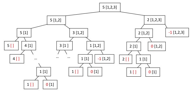
As can be seen from the above diagram, this algorithm too can benefit from memoization. Try it at home!
Quicksort
def slowsort(lst):
    """quicksort of list lst"""
    if len(lst) <= 1:
        return lst
    pivot = lst[0]      # select first element from list
    smaller = [elem for elem in lst if elem < pivot]
    equal = [elem for elem in lst if elem == pivot]
    greater = [elem for elem in lst if elem > pivot]
    return slowsort(smaller) + equal + slowsort(greater)
import random

def quicksort(lst):
    """quicksort of list lst"""
    if len(lst) <= 1:
        return lst
    pivot = random.choice(lst) # select a random element from list
    smaller = [elem for elem in lst if elem < pivot]
    equal = [elem for elem in lst if elem == pivot]
    greater = [elem for elem in lst if elem > pivot]
    return quicksort(smaller) + equal + quicksort(greater)
Running time on random input
lst = [random.randint(0,100) for _ in range(100000)]
%timeit -n 10 slowsort(lst)
10 loops, best of 3: 143 ms per loop
%timeit -n 10 quicksort(lst)
10 loops, best of 3: 150 ms per loop
lst = [i for i in range(100)]
%timeit -n 10 slowsort(lst)
10 loops, best of 3: 2.55 ms per loop
%timeit -n 10 quicksort(lst)
10 loops, best of 3: 816 us per loop
Complexity
Assume the values are unique (what will happen if all values are the same?, i.e. lst = [1, 1, 1, 1, ..., 1]).
- At the first function call, you go over the entire list and separate the numbers that are smaller and bigger than the pivot. So this is $O(n)$.
- At the next function calls, you go over two sub-lists and do the same for them, and the total of items in the two sub-lists is $n$, so this is also $O(n)$.
- This goes on until we reach lists of length 1
- Denoting the recursion depth by x, the complexity is therefore $O(n x)$.
For Slowsort, the worst case is when the list is already sorted ([1,2,3,4,5]) in which case the pivot will always be the minimum and the sub-lists will always be of length 1 and *k-1$.
The recursion depth will be $n$ and therefore the complexity $O(n^2)$.
In the base case, however, the pivot is always the median, and therefore the sub-lists are always of equal size, making for a recursion depth of $\log_2{n}$ and complexity of $O(n \log{n})$.
For Quicksort the choice of the pivot is random, so the algorithm complexity does not depend on the input order.
On average, the pivot will be the median (which is the best choice), the sub-lists will be of equal size, and the recursion depth will be $\log_2{n} \;$ leading to a complexity of $O(n \log{n})$.
Fin
This notebook is part of the Extended introduction to computer science course at Tel-Aviv University.
The notebook was written using Python 3.2 and IPython 0.13.1.
The code is available at https://raw.github.com/yoavram/CS1001.py/master/recitation6.ipynb.
The notebook can be viewed online at http://nbviewer.ipython.org/urls/raw.github.com/yoavram/CS1001.py/master/recitation6.ipynb.
This work is licensed under a Creative Commons Attribution-ShareAlike 3.0 Unported License.