3. Numpy.
3.1. Descripción.
- Python tiene listas, enteros, punto flotante, etc. Para cálculo numérico necesitamos más... allí aparece Numpy.
- Numpy es un paquete que provee a Python con arreglos multidimensionales de alta eficiencia y diseñados para cálculo científico.
- Un array puede contener:
- tiempos discretos de un experimento o simulación.
- señales grabadas por un instrumento de medida.
- pixeles de una imagen, etc.
%matplotlib inline
import numpy as np
3.2. El objeto arreglo.
- Los arreglos de NumPy son de tipado estático y homogéneo.
- Son más eficientes en el uso de la memoria.
- La funciones matemáticas complejas y computacionalmente costosas (pj: la multiplicación de matrices) son implementadas en lenguajes compilados como C o Fortran.
3.2.1. Creación de arreglos unidimensionales.
A partir de una lista de Python:
lista = [1, 2, 3, 4 , 5]
type(lista)
list
a = np.array(lista)
a
array([1, 2, 3, 4, 5])
type(a)
numpy.ndarray
Podemos conocer el tipo de datos a través de dtype:
a.dtype
dtype('int64')
Incluso podemos definir el tipo de dato al momento de la creación de arreglo:
a_complejo = np.array(lista, dtype=complex)
a_complejo
array([ 1.+0.j, 2.+0.j, 3.+0.j, 4.+0.j, 5.+0.j])
a_complejo.dtype
dtype('complex128')
o cambiar el tipo de dato:
a_no_mas_complejo = a_complejo.astype(np.int64)
-c:1: ComplexWarning: Casting complex values to real discards the imaginary part
a_no_mas_complejo
array([1, 2, 3, 4, 5])
Si queremos ver algunas características del arreglo a:
a.ndim # dimensión
1
a.shape # 5 x 1
(5,)
len(a) # elementos en la primera dimension
5
3.2.2. Creación de arreglos de 2 y 3 dimensiones.
b = np.array([[0, 1, 2], [3, 4, 5]]) # arreglo 2 x 3
b
array([[0, 1, 2],
       [3, 4, 5]])
b.ndim
2
b.shape
(2, 3)
len(b) # elementos en la primera dimensión
2
c = np.array([[[1], [2]], [[3], [4]]])
c
array([[[1],
        [2]],

       [[3],
        [4]]])
c.shape
(2, 2, 1)
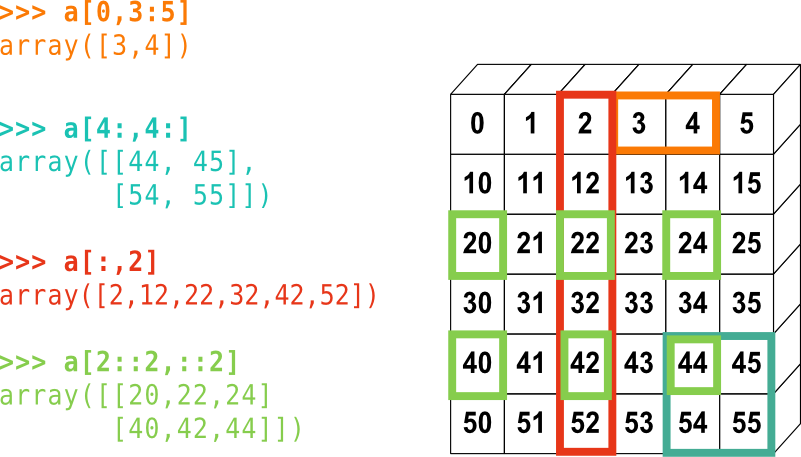
3.2.3. Indexado.
a = np.arange(10) # otra forma de generar un arreglo: a través de funciones específicas de numpy
a
array([0, 1, 2, 3, 4, 5, 6, 7, 8, 9])
a[0], a[2], a[-1]
(0, 2, 9)
mis_indices = [0, 2, -1] # puedo listar índices
a[mis_indices] # y luego indexar por esa lista ("fancy indexing")
array([0, 2, 9])
3.2.4. Cortes.
a
array([0, 1, 2, 3, 4, 5, 6, 7, 8, 9])
a[2:9] # corta en intervalos
array([2, 3, 4, 5, 6, 7, 8])
a[2:9:3] # puedo especificar cada cuánto cortar
array([2, 5, 8])
a[::2]
array([0, 2, 4, 6, 8])
a[3::2]
array([3, 5, 7, 9])
a[-2:]
array([8, 9])
Un esquema siempre ayuda...
3.2.5. Copias y Vistas.
Si copiamos una lista en Python... si modificamos la copia, no se modifica la lista originalmente copiada:
%%python
# python cell magic, lindo... no?
a = [1, 2, 3]
b = a[:]
print b
b[0] = 100
print b
print a
[1, 2, 3]
[100, 2, 3]
[1, 2, 3]
Si trabajamos con arreglos de NumPy, el comportamiento es diferente (cuando copiamos, en realidad, estamos haciendo una vista al objeto original, apuntamos al mismo objeto):
a = np.array([1, 2, 3])
b = a[:]
print b
b[0] = 100
print b
print a
[1 2 3]
[100   2   3]
[100   2   3]
¿Cómo resolvemos esta discrepancia?
a = np.array([1, 2, 3])
b = a[:].copy() # fuerzo la copia
print b
b[0] = 100
print b
print a
[1 2 3]
[100   2   3]
[1 2 3]
3.3. Operaciones numéricas sobre arreglos.
3.3.1. Operaciones por elementos.
Escalares:
a = np.array([1, 2, 3, 4])
a + 1
array([2, 3, 4, 5])
2**a
array([ 2, 4, 8, 16])
Aritméticas:
b = np.ones(4) # otra función generadora de arreglos
b = b + 1
b
array([ 2., 2., 2., 2.])
b - a
array([ 1., 0., -1., -2.])
a * b
array([ 2., 4., 6., 8.])
c = np.ones((3, 3))
c
array([[ 1.,  1.,  1.],
       [ 1.,  1.,  1.],
       [ 1.,  1.,  1.]])
c * c # ojo! esto es una multiplicación elemento por elemento.
array([[ 1.,  1.,  1.],
       [ 1.,  1.,  1.],
       [ 1.,  1.,  1.]])
c.dot(c) # multiplicación matricial
array([[ 3.,  3.,  3.],
       [ 3.,  3.,  3.],
       [ 3.,  3.,  3.]])
Lógicas:
a = np.array([1, 2, 3, 4])
b = np.array([4, 2, 2, 4])
a == b
array([False, True, False, True], dtype=bool)
a > b
array([False, False, True, False], dtype=bool)
Otras operaciones lógicas:
a = np.array([1, 1, 0, 0], dtype=bool)
b = np.array([1, 0, 1, 0], dtype=bool)
a | b # or, np.logical_or
array([ True, True, True, False], dtype=bool)
a & b # and, np.logical_and
array([ True, False, False, False], dtype=bool)
a ^ b # xor, np.logical_xor
array([False, True, True, False], dtype=bool)
not_a = - a # not, np.logical_not
not_a
array([False, False, True, True], dtype=bool)
3.3.2. Reducciones básicas.
Calculando sumas:
x = np.array([1, 2, 3, 4])
x.sum() # np.sum(x)
10
por filas y columnas:
x = np.array([[1, 1], [2, 2]])
x.sum(axis=0) # por columna
array([3, 3])
x[:,0].sum(), x[:,1].sum()
(3, 3)
x.sum(axis=1) # por filas
array([2, 4])
x[0,:].sum(), x[1,:].sum()
(2, 4)
Calculando estadísticos:
x = np.array([1, 2, 3, 1])
x.mean()
1.75
x.std()
0.82915619758884995
x.std(ddof=1) # con divisor n - 1
0.9574271077563381
np.median(x)
1.5
y = np.array([[1, 2, 3], [5, 6, 1]])
np.median(y, axis=-1) # último eje: en este caso, filas
array([ 2., 5.])
Encontrando extremos:
x.min()
1
np.argmin(x) # índice del mínimo
0
x.max()
3
np.argmax(x) # índice del máximo
2
Más operaciones lógicas:
np.all([True, True, False])
False
np.any([True, True, False])
True
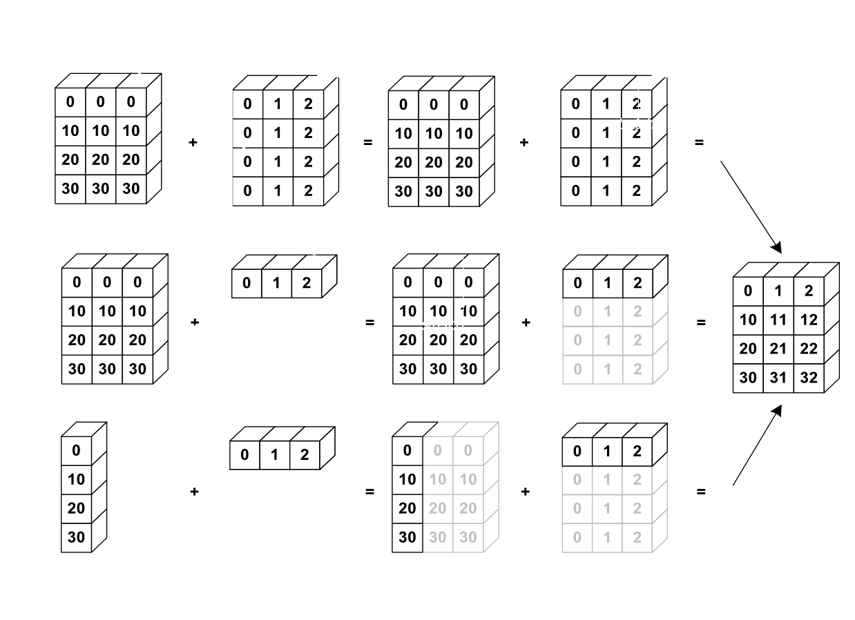
3.3.3. Broadcasting.
En NumPy es posible hacer operaciones entre arreglos de diferente tamaño a través del broadcasting.
- NumPy transforma (propaga) los arreglos involucrados para que tengan el mismo tamaño y, por tanto, puedan someterse a las operaciones por elementos sin generar excepciones.
a = np.arange(0, 40, 10)
a.shape
(4,)
a = a[:, np.newaxis]  # suma un nuevo eje (arreglo 2D)
a.shape
a
array([[ 0],
       [10],
       [20],
       [30]])
b = np.array([0, 1, 2])
b
array([0, 1, 2])
a + b
array([[ 0,  1,  2],
       [10, 11, 12],
       [20, 21, 22],
       [30, 31, 32]])
3.3.4. Álgebra lineal básica.
Multiplicaión de matrices:
a = np.triu(np.ones((3, 3)), 1)   # see help(np.triu)
a
array([[ 0.,  1.,  1.],
       [ 0.,  0.,  1.],
       [ 0.,  0.,  0.]])
b = np.diag([1, 2, 3])
b
array([[1, 0, 0],
       [0, 2, 0],
       [0, 0, 3]])
a.dot(b)
array([[ 0.,  2.,  3.],
       [ 0.,  0.,  3.],
       [ 0.,  0.,  0.]])
Trasposición:
a.T
array([[ 0.,  0.,  0.],
       [ 1.,  0.,  0.],
       [ 1.,  1.,  0.]])
Inversión y resolución de equaciones lineales:
A = a + b
A
array([[ 1.,  1.,  1.],
       [ 0.,  2.,  1.],
       [ 0.,  0.,  3.]])
B = np.linalg.inv(A)
B
array([[ 1.        , -0.5       , -0.16666667],
       [ 0.        ,  0.5       , -0.16666667],
       [ 0.        ,  0.        ,  0.33333333]])
B.dot(A)
array([[ 1.,  0.,  0.],
       [ 0.,  1.,  0.],
       [ 0.,  0.,  1.]])
x = np.linalg.solve(A, [1, 2, 3])
x
array([-0.5, 0.5, 1. ])
A.dot(x)
array([ 1., 2., 3.])
Cálculo de autovalores:
np.linalg.eigvals(A)
array([ 1., 2., 3.])
3.4. Manipulación de arreglos.
3.4.1. Manipulación de la forma de los arreglos.
"Aplanado":
a = np.array([[1, 2, 3], [4, 5, 6]])
a.ravel()
array([1, 2, 3, 4, 5, 6])
a.T
array([[1, 4],
       [2, 5],
       [3, 6]])
a.T.ravel()
array([1, 4, 2, 5, 3, 6])
Cambio de forma:
a.shape
(2, 3)
b = a.ravel()
b
array([1, 2, 3, 4, 5, 6])
b.reshape((2,3))
array([[1, 2, 3],
       [4, 5, 6]])
a = np.arange(36)
b = a.reshape((6,6))
b
array([[ 0,  1,  2,  3,  4,  5],
       [ 6,  7,  8,  9, 10, 11],
       [12, 13, 14, 15, 16, 17],
       [18, 19, 20, 21, 22, 23],
       [24, 25, 26, 27, 28, 29],
       [30, 31, 32, 33, 34, 35]])
b = a.reshape((6, -1)) # -1: comodín, se infiere
b
array([[ 0,  1,  2,  3,  4,  5],
       [ 6,  7,  8,  9, 10, 11],
       [12, 13, 14, 15, 16, 17],
       [18, 19, 20, 21, 22, 23],
       [24, 25, 26, 27, 28, 29],
       [30, 31, 32, 33, 34, 35]])
Cambio de tamaño:
a = np.arange(4)
a.resize((8,))
a
array([0, 1, 2, 3, 0, 0, 0, 0])
Agregado de nuevas dimensiones:
vector = np.array([1,2,3])
vector
array([1, 2, 3])
np.shape(vector)
(3,)
matrix_col = vector[:, np.newaxis] # lo convierto en matrix 3 x 1
matrix_col
array([[1],
       [2],
       [3]])
np.shape(matrix_col)
(3, 1)
matrix_ver = vector[np.newaxis, :] # lo convierto en matrix 1 x 3
matrix_ver
array([[1, 2, 3]])
np.shape(matrix_ver)
(1, 3)
Repeticiones:
a = np.array([[1, 2], [3, 4]])
a
array([[1, 2],
       [3, 4]])
np.repeat(a, 3)
array([1, 1, 1, 2, 2, 2, 3, 3, 3, 4, 4, 4])
np.tile(a, 3)
array([[1, 2, 1, 2, 1, 2],
       [3, 4, 3, 4, 3, 4]])
Concatenación:
b = np.array([[5, 6]])
np.concatenate((a, b), axis=0)
array([[1, 2],
       [3, 4],
       [5, 6]])
np.concatenate((a, b.T), axis=1)
array([[1, 2, 5],
       [3, 4, 6]])
np.vstack((a,b))
array([[1, 2],
       [3, 4],
       [5, 6]])
np.hstack((a,b.T))
array([[1, 2, 5],
       [3, 4, 6]])
3.4.2. Funciones para tomar datos de los arreglos.
a = np.array([1,0,1,0,0], dtype=bool)
b = np.where(a) # where
b
(array([0, 2]),)
a = np.array([[1, 2, 3], [4, 5, 6], [7, 8, 9]])
a
array([[1, 2, 3],
       [4, 5, 6],
       [7, 8, 9]])
np.diag(a) # diag
array([1, 5, 9])
a = np.arange(10,16)
a
array([10, 11, 12, 13, 14, 15])
indices = [1, 3, 5]
np.take(a, indices)
array([11, 13, 15])
which = [0, 0, 1, 0]
choices = [[-2, -3, -4, -5], [5, 6, 7, 8]]
np.choose(which, choices)
array([-2, -3, 7, -5])
3.4.3. Funciones generadoras de arreglos.
x = np.arange(0, 10, 1) # argumentos: inicio, fin, paso
x
array([0, 1, 2, 3, 4, 5, 6, 7, 8, 9])
np.linspace(0, 10, 25) # incio, fin, n° puntos intermedios
array([  0.        ,   0.41666667,   0.83333333,   1.25      ,
         1.66666667,   2.08333333,   2.5       ,   2.91666667,
         3.33333333,   3.75      ,   4.16666667,   4.58333333,
         5.        ,   5.41666667,   5.83333333,   6.25      ,
         6.66666667,   7.08333333,   7.5       ,   7.91666667,
         8.33333333,   8.75      ,   9.16666667,   9.58333333,  10.        ])
np.logspace(0, 10, 10, base=np.e)
array([  1.00000000e+00,   3.03773178e+00,   9.22781435e+00,
         2.80316249e+01,   8.51525577e+01,   2.58670631e+02,
         7.85771994e+02,   2.38696456e+03,   7.25095809e+03,
         2.20264658e+04])
x, y = np.mgrid[0:5, 0:5] # similar al meshgrid de MATLAB
x
array([[0, 0, 0, 0, 0],
       [1, 1, 1, 1, 1],
       [2, 2, 2, 2, 2],
       [3, 3, 3, 3, 3],
       [4, 4, 4, 4, 4]])
y
array([[0, 1, 2, 3, 4],
       [0, 1, 2, 3, 4],
       [0, 1, 2, 3, 4],
       [0, 1, 2, 3, 4],
       [0, 1, 2, 3, 4]])
np.random.rand(5, 5) # números aleatorios uniformes [0,1]
array([[ 0.71993812,  0.05176951,  0.37876399,  0.71104661,  0.09103074],
       [ 0.66332802,  0.56448753,  0.6795584 ,  0.19281203,  0.62263155],
       [ 0.96436095,  0.06478416,  0.05179043,  0.391897  ,  0.96105272],
       [ 0.05728427,  0.55147176,  0.3245483 ,  0.25468026,  0.66221203],
       [ 0.55938751,  0.5883277 ,  0.9253775 ,  0.27429514,  0.3440919 ]])
np.random.randn(5,5) # números aleatorios normalmente distribuidos
array([[-0.65733   , -0.39731405,  1.7341414 ,  0.3567832 ,  1.69461793],
       [ 1.54425562, -1.82893025, -0.15648911,  0.66672057,  0.66853341],
       [ 0.83117805,  1.17071038, -0.81596502,  0.5750493 , -0.63990098],
       [-0.56259403,  0.45052975, -0.43402709, -0.40855709, -0.70216341],
       [-0.58823829, -1.05708393,  1.21155867,  0.84643448,  2.0027709 ]])
np.diag([1,2,3]) # matrix diagonal
array([[1, 0, 0],
       [0, 2, 0],
       [0, 0, 3]])
np.diag([1,2,3], k=1) # desplazamiento sobre la diagonal
array([[0, 1, 0, 0],
       [0, 0, 2, 0],
       [0, 0, 0, 3],
       [0, 0, 0, 0]])
np.zeros((3,3))
array([[ 0.,  0.,  0.],
       [ 0.,  0.,  0.],
       [ 0.,  0.,  0.]])
np.ones((3,3))
array([[ 1.,  1.,  1.],
       [ 1.,  1.,  1.],
       [ 1.,  1.,  1.]])
3.4.4. Entrada/Salida
Podemos leer archivos csv:
!head stockholm_td_adj.dat
1800  1  1    -6.1    -6.1    -6.1 1
1800  1  2   -15.4   -15.4   -15.4 1
1800  1  3   -15.0   -15.0   -15.0 1
1800  1  4   -19.3   -19.3   -19.3 1
1800  1  5   -16.8   -16.8   -16.8 1
1800  1  6   -11.4   -11.4   -11.4 1
1800  1  7    -7.6    -7.6    -7.6 1
1800  1  8    -7.1    -7.1    -7.1 1
1800  1  9   -10.1   -10.1   -10.1 1
1800  1 10    -9.5    -9.5    -9.5 1
data = np.genfromtxt('stockholm_td_adj.dat')
data.shape
(77431, 7)
data
array([[  1.80000000e+03,   1.00000000e+00,   1.00000000e+00, ...,
         -6.10000000e+00,  -6.10000000e+00,   1.00000000e+00],
       [  1.80000000e+03,   1.00000000e+00,   2.00000000e+00, ...,
         -1.54000000e+01,  -1.54000000e+01,   1.00000000e+00],
       [  1.80000000e+03,   1.00000000e+00,   3.00000000e+00, ...,
         -1.50000000e+01,  -1.50000000e+01,   1.00000000e+00],
       ...,
       [  2.01100000e+03,   1.20000000e+01,   2.90000000e+01, ...,
          4.20000000e+00,   4.20000000e+00,   1.00000000e+00],
       [  2.01100000e+03,   1.20000000e+01,   3.00000000e+01, ...,
         -1.00000000e-01,  -1.00000000e-01,   1.00000000e+00],
       [  2.01100000e+03,   1.20000000e+01,   3.10000000e+01, ...,
         -3.30000000e+00,  -3.30000000e+00,   1.00000000e+00]])
pero también podemos escribirlos:
M = np.random.rand(3,3)
M
array([[ 0.12192489,  0.5600679 ,  0.98467243],
       [ 0.91231303,  0.75122357,  0.54310547],
       [ 0.18771526,  0.33981397,  0.48772906]])
np.savetxt("random-matrix.csv", M)
!cat random-matrix.csv
1.219248903542134999e-01 5.600678957725345741e-01 9.846724267415249976e-01
9.123130259426238675e-01 7.512235706886890574e-01 5.431054672782125170e-01
1.877152580076981714e-01 3.398139715902742664e-01 4.877290607674301670e-01
np.savetxt("random-matrix.csv", M, fmt='%.5f') # fmt especifica el formato a escribir
!cat random-matrix.csv
0.12192 0.56007 0.98467
0.91231 0.75122 0.54311
0.18772 0.33981 0.48773
np.save("random-matrix.npy", M)
!file random-matrix.npy
random-matrix.npy: data
np.load("random-matrix.npy")
array([[ 0.12192489,  0.5600679 ,  0.98467243],
       [ 0.91231303,  0.75122357,  0.54310547],
       [ 0.18771526,  0.33981397,  0.48772906]])