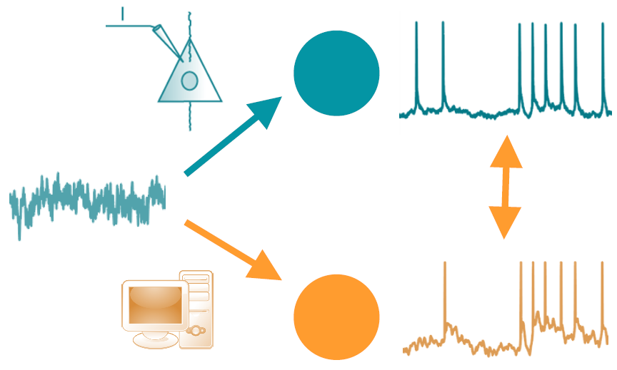
Spiking neuron models can accurately reproduce the response to a somatically injected current
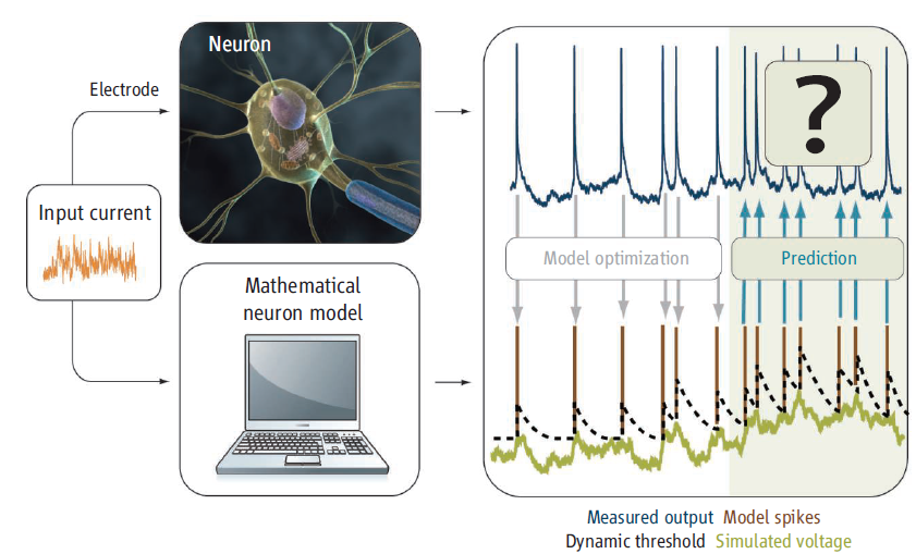
How to estimate the parameters?
- Model-specific optimization algorithms
- Generic optimization with Brian
The BRIAN model fitting toolbox
- Give the equations in mathematical form as usual
- Specify the parameters to optimize
- Specify the injected current and the output spikes
- Run the procedure and get the optimized parameters
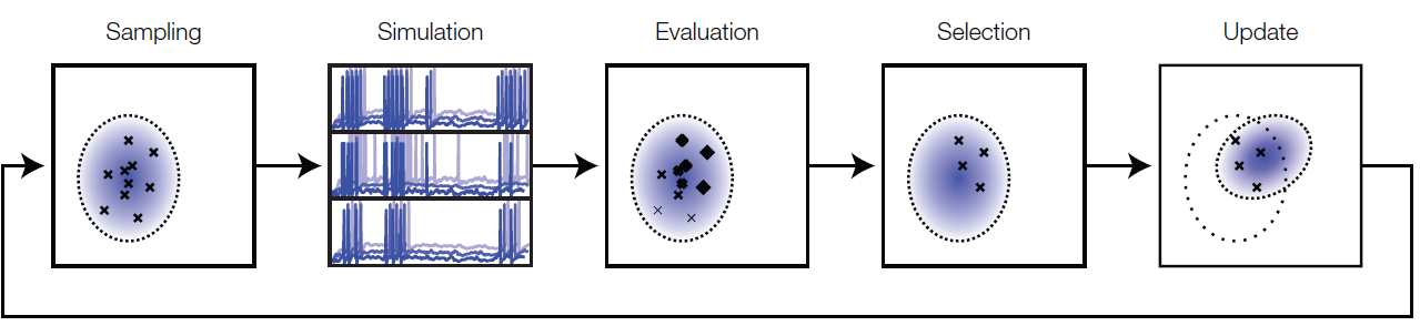
How it works
- The model is simulated with Brian: one neuron = one parameter set
- The best parameters are found with a stochastic global optimization algorithm (e.g. CMA-ES)
Getting started
You need Brian (it includes directly the model fitting library).
You also need Playdoh (distributed optimization) (github.com/rossant/playdoh):
pip install playdoh
Toy example
- Let's first simulate a simple integrate-and-fire neuron responding to an injected fluctuating current.
In [1]:
%pylab inline
Welcome to pylab, a matplotlib-based Python environment [backend: module://IPython.kernel.zmq.pylab.backend_inline].
For more information, type 'help(pylab)'.
In [2]:
from brian import *
from brian.library.modelfitting import *
from brian.library.random_processes import *
D:\SVN\Brian\brian\utils\sparse_patch\__init__.py:39: UserWarning: Couldn't find matching sparse matrix patch for scipy version 0.12.0, but in most cases this shouldn't be a problem.
  warnings.warn("Couldn't find matching sparse matrix patch for scipy version %s, but in most cases this shouldn't be a problem." % scipy.__version__)
In [3]:
R, tau = 1., 5 * ms
eqs = Equations('''dV/dt=(R*I-V)/tau : 1''')
eqs += OrnsteinUhlenbeck('I',
        mu=.5, sigma=.5, tau=5 * ms)
In [4]:
G = NeuronGroup(N=1, model=eqs, reset=0., threshold=1., refractory=5 * ms)
Mspikes = SpikeMonitor(G)
Vstate = StateMonitor(G, 'V', record=True)
Istate = StateMonitor(G, 'I', record=True)
net = Network(G, Mspikes, Vstate, Istate)
reinit_default_clock()
net.run(1 * second)
In [5]:
figure(figsize=(10,4))
Vif, current, spikes = Vstate[0], Istate[0], Mspikes.spiketimes[0]
plot(Vstate.times, Vif, '-k');
vlines(spikes, 1, 3);

- Now, let's fit the same model on the simulated data.
In [6]:
equations = Equations('''
    dV/dt=(R*I-V)/tau : 1
    I : 1
    R : 1
    tau : second
''')
In [7]:
results = modelfitting(model=equations,
    reset=0, threshold=1,
    data=spikes, input=current, dt=defaultclock.dt,
    popsize=250, maxiter=10, cpu=1,
    R=[0., 10.], tau=[2*ms, 50*ms],
    refractory=[0*ms, 10*ms])
In [8]:
print_table(results)
RESULTS
--------------------------------
R                  1.102
refractory         2.576e-3
tau                7.300e-3
best fit           1.000
Let's compare the actual and fitted traces and spikes.
In [9]:
G = NeuronGroup(N=1, model=eqs, reset=0.,
    threshold=1.,
    refractory=results[0]['refractory'] * second)
reinit_default_clock()
G.I = TimedArray(current)
G.R, G.tau = results[0]['R'], results[0]['tau']
Mspikes = SpikeMonitor(G)
Vstate = StateMonitor(G, 'V', record=True)
Istate = StateMonitor(G, 'I', record=True)
net = Network(G, Mspikes, Vstate, Istate)
net.run(1 * second)
In [10]:
figure(figsize=(10,4))
V_fit, spikes_fit = Vstate[0], Mspikes.spiketimes[0]
plot(Vstate.times, Vif, 'k');
vlines(spikes, 1, 3, color='k');
plot(Vstate.times, V_fit, '-r');
vlines(spikes_fit, 1, 3, color='r');

Fitting an IF neuron to real data
- Let's get the data from the Brian repository.
- These come from patch-clamp recordings in neurons from mouse auditory cortex, performed by Anna K. Magnusson.
In [11]:
import urllib2
path = 'https://neuralensemble.org/svn/brian/trunk/examples/modelfitting/'
# These files were saved with `numpy.savetxt`.
current = np.fromstring(
    urllib2.urlopen(path + 'current.txt').read(),
    sep='\n')
spikes = np.fromstring(
    urllib2.urlopen(path + 'spikes.txt').read(),
    sep='\n')
What does the data look like?
In [12]:
t = arange(current.size) * defaultclock.dt
figure(figsize=(10,4));
subplot(211);
plot(t, current, '-b');
subplot(212);
hlines([0], 0, 1);
vlines(spikes, 0, 1);
ylim(-.5, 1.5);

Let's fit an IF neuron with an adaptive threshold.
In [13]:
eqs = Equations('''
    dV/dt=(R*I-V)/tau : volt
    dVt/dt=(a*V-Vt)/taut : volt
    I : amp
    R : ohm
    a : 1
    alpha : volt
    tau : second
    taut : second
''')
threshold = '''(V>1+Vt)'''
reset = '''
V = 0
Vt += alpha
'''
In [14]:
results = modelfitting(model=eqs,
    reset=reset, threshold=threshold,
    data=spikes, input=current, dt=defaultclock.dt,
    popsize=500, maxiter=5, cpu=4,
    R=[10*Mohm, 10*Mohm, 10000.*Mohm, 10000.*Mohm],
    a=[0., 1.], alpha=[0., 20.*mV],
    tau=[2*ms, 50*ms], taut=[20*ms, 200*ms])
In [15]:
print_table(results)
RESULTS
--------------------------------
R                  2.997e+9
a                  0.306
alpha              7.566e-3
tau               20.226e-3
taut              53.760e-3
best fit           0.875
Let's simulate the model with the fitted parameters.
In [16]:
G = NeuronGroup(N=1, model=eqs, reset=reset,
    threshold=threshold,)
reinit_default_clock()
G.I = TimedArray(current)
for key, val in results[0].best_pos.iteritems():
    setattr(G, key, val)
Mspikes = SpikeMonitor(G)
Vstate = StateMonitor(G, 'V', record=True)
Vtstate = StateMonitor(G, 'Vt', record=True)
Istate = StateMonitor(G, 'I', record=True)
net = Network(G, Mspikes, Vstate, Vtstate, Istate)
net.run(1 * second)
brian.equations   : WARNING  Equation variable R also exists in the namespace
WARNING:brian.equations:Equation variable R also exists in the namespace
brian.equations   : WARNING  Equation variable tau also exists in the namespace
WARNING:brian.equations:Equation variable tau also exists in the namespace
In [17]:
figure(figsize=(10,4))
V_fit, Vt_fit, spikes_fit = Vstate[0], Vtstate[0], Mspikes.spiketimes[0]
plot(Vstate.times, V_fit, 'r');
plot(Vstate.times, 1 + Vt_fit, 'g');
vlines(spikes, 1 + Vt_fit[(spikes * 1000).astype(int)], 3, color='k');
vlines(spikes_fit, 1 + Vt_fit[(spikes_fit * 1000).astype(int)], 3, color='r');

Reducing a biophysical model to a spiking model
We first simulate a Hodgkin-Huxley model with an input current.
In [18]:
area = 20000*umetre**2
Cm = (1*ufarad*cm**-2)*area
gl = (5e-5*siemens*cm**-2)*area
El = -60*mV
EK = -90*mV
ENa = 50*mV
g_na = (100*msiemens*cm**-2)*area
g_kd = (30*msiemens*cm**-2)*area
VT = -63*mV
eqs = Equations('''
dv/dt = (gl*(El-v)+I-\
    g_na*(m*m*m)*h*(v-ENa)-\
    g_kd*(n*n*n*n)*(v-EK))/Cm : volt
dm/dt = alpham*(1-m)-betam*m : 1
dn/dt = alphan*(1-n)-betan*n : 1
dh/dt = alphah*(1-h)-betah*h : 1
alpham = 0.32*(mV**-1)*(13*mV-v+VT)/ \
    (exp((13*mV-v+VT)/(4*mV))-1.)/ms : Hz
betam = 0.28*(mV**-1)*(v-VT-40*mV)/ \
    (exp((v-VT-40*mV)/(5*mV))-1)/ms : Hz
alphah = 0.128*exp((17*mV-v+VT)/(18*mV))/ms : Hz
betah = 4./(1+exp((40*mV-v+VT)/(5*mV)))/ms : Hz
alphan = 0.032*(mV**-1)*(15*mV-v+VT)/ \
    (exp((15*mV-v+VT)/(5*mV))-1.)/ms : Hz
betan = .5*exp((10*mV-v+VT)/(40*mV))/ms : Hz
I : amp
''')
In [19]:
G = NeuronGroup(1, model=eqs, threshold=EmpiricalThreshold(threshold=-20*mV, refractory=3*ms),
              implicit=True, freeze=True)
reinit_default_clock()
current -= mean(current)
current = 1.0e-10 + 10.0e-1 * current
G.I = TimedArray(current)
Mspikes = SpikeMonitor(G)
Vstate = StateMonitor(G, 'v', record=True)
net = Network(G, Mspikes, Vstate)
net.run(1 * second)
In [20]:
figure(figsize=(10,4))
Vhh, spikes = Vstate[0], Mspikes.spiketimes[0]
plot(Vstate.times, Vhh, '-k');

Now, let's fit an adaptive integrate-and-fire on this model to "reduce" the complex biophysical model to a simpler phenomenological model.
In [21]:
eqs = Equations('''
    dV/dt=(R*I-V)/tau : volt
    dVt/dt=(a*V-Vt)/taut : volt
    I : amp
    R : ohm
    a : 1
    alpha : volt
    tau : second
    taut : second
''')
threshold = '''(V>1+Vt)'''
reset = '''
V = 0
Vt += alpha
'''
In [36]:
results = modelfitting(model=eqs,
    reset=reset, threshold=threshold,
    data=spikes, input=current, dt=defaultclock.dt,
    popsize=500, maxiter=5, cpu=4,
    R=[10*Mohm, 10*Mohm, 10000.*Mohm, 10000.*Mohm],
    a=[0., 1.], alpha=[0., 0., 20.*mV, 20.*mV],
    tau=[2*ms, 50*ms], taut=[20*ms, 200*ms])
Here are the results
In [37]:
print_table(results)
RESULTS
--------------------------------
R                  9.414e+9
a                  0.299
alpha             12.688e-3
tau               21.821e-3
taut               0.156
best fit           0.488
In [38]:
G = NeuronGroup(N=1, model=eqs, reset=reset,
    threshold=threshold,)
reinit_default_clock()
G.I = TimedArray(current)
for key, val in results[0].best_pos.iteritems():
    setattr(G, key, val)
Mspikes = SpikeMonitor(G)
Vstate = StateMonitor(G, 'V', record=True)
Vtstate = StateMonitor(G, 'Vt', record=True)
Istate = StateMonitor(G, 'I', record=True)
net = Network(G, Mspikes, Vstate, Vtstate, Istate)
net.run(1 * second)
In [39]:
figure(figsize=(10,4))
V_fit, Vt_fit, spikes_fit = Vstate[0], Vtstate[0], Mspikes.spiketimes[0]
plot(Vstate.times, 2+Vhh*20, 'k');
plot(Vstate.times, V_fit, 'r');
plot(Vstate.times, 1 + Vt_fit, 'g');
vlines(spikes_fit, 1 + Vt_fit[(spikes_fit * 1000).astype(int)], 3, color='r');
