Exploring Jupyter Notebook
Mark Santcroos, Department of Human Genetics, Leiden University Medical Center
Examples and ideas taken from: Jupyter Documentation, The role of computing in science, and an earlier version of this lecture by Michiel van Galen.
Introduction
Requirements on scientific computing
"High-profile journals have called for increased openness in computational sciences. Some prestigious journals, including Science, have even started to demand of authors to provide the source code for simulation software used in publications to readers upon request."
Reproducible Research in Computational Science, Roger D. Peng, Science 334, 1226 (2011).
Shining Light into Black Boxes, A. Morin et al., Science 336, 159-160 (2012).
The case for open computer programs, D.C. Ince, Nature 482, 485 (2012).
The cornerstone of the scientific method
- Replication & Reproduction
To achieve this in scientific computing (programming)
Any source code which generates data should be:
- Tracked! (e.g. git)
- Backed up and secured
- Ideally published online
- Additionally: Also track external software versions and settings
Jupyter Notebook to the rescue
"Web-based interactive computational environment where you can combine code execution, text, mathematics, plots and rich media into a single document."
Multiple ways to launch python
- python (interactive)
- python script.py
- ipython
- IDE (integrated development environment), e.g. Spyder
- Jupyter notebook (used to be called ipython notebook)
What is it?
- Cell based executable workflow
- Interactive computational documents
- Add elegant explanatory text
- Direct output of computations
- Add figures and video
- Integration in Git
- Export your notebooks to PDF or HTML (nbconvert)
- Share notebooks easily with nbviewer or LUMC Gitlab
The notebook user interface
- Cell based workflow
- Move between cells with the arrow keys or clicks with the mouse
There are two different modes from which always one is active
- Edit mode
- Hit ENTER or click the edit area to change to edit mode
- Indicated with a blue cell border
- Edit your cell as if a normal text editor
- Command mode
- Hit ESCAPE to change into command mode
- Indicated with a grey cell border
- Edit the notebook as a whole
Shortcuts
Note: Different shortcuts apply in both modes!
Edit mode shortcuts:
- esc : command mode
- shift+enter : run cell, select below
- ctrl+enter : run cell
Command mode shortcuts
enter : edit mode
shift+enter : run cell
ctrl+enter : run cell, select below
y : to code
m : to markdown
k : move cell up
j : move cell down
a : insert cell above
b : insert cell below
x : cut cell
c : copy cell
v : paste cell below
z : undo last delete
d : delete cell (press twice)
Press 'h' to show the help.
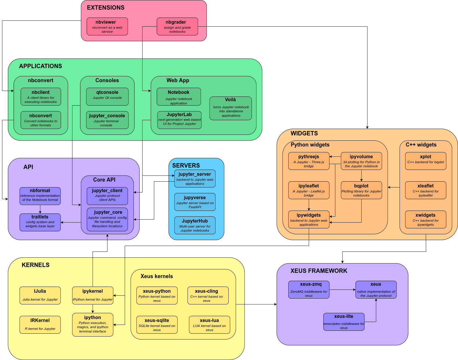
Architecture
Installation
- Official Installing Jupyter Procedure
- We already have it, it comes shipped with Anaconda
### !! Exercise !!
###
### Launch Jupyter on your own machine, and create a new notebook
###
Cells
Two different cell types:
- Code cell
- Contains code
- Inline comments
- Python or system calls
# This is a code cell
z = 42
### !! Exercise !!
###
### Create a code cell and run some code
###
- Markdown cell
- Format your notebook
This is a markdown cell which allows to format your document nicely and add context to code cells.
Set the cell type of the selected cell
- Select the type from the dropdown box in the toolbar
- In command mode only: Press 'y' for code or 'm' for markdown
Code cells
- Any piece of python code can be ran.
- The result is persistent.
- Cells can be executed in artibrary order.
Auto-completion
import numpy
# numpy.rand <TAB>
numpy.random.random()
0.9573042214012784
# numpy.random <SHIFT-TAB>
numpy.random
# Type:        module
# String form: <module 'numpy.random' from '/Users/mark/anaconda/lib/python2.7/site-packages/numpy/random/__init__.pyc'>
# File:        ~/anaconda/lib/python2.7/site-packages/numpy/random/__init__.py
<module 'numpy.random' from '/home/mihai/.pyenv/versions/3.8.5/lib/python3.8/site-packages/numpy/random/__init__.py'>
### !! Exercise !!
###
### Explore tab completion on your (less) favourite library (function)
###
Output
- When a cell is run it can generate output
- This is shown below the cell in the output area
- Output is asynchronous
- Outputs are objects and the last one is available under the variable '_'
23 + 19
42
print(f"The Answer to the Ultimate Question of Life, the Universe, and Everything is {_}.")
The Answer to the Ultimate Question of Life, the Universe, and Everything is 42.
- Output can be toggled on/off.
#
# All output
#
for n in range(100): print(n)
0
1
2
3
4
5
6
7
8
9
10
11
12
13
14
15
16
17
18
19
20
21
22
23
24
25
26
27
28
29
30
31
32
33
34
35
36
37
38
39
40
41
42
43
44
45
46
47
48
49
50
51
52
53
54
55
56
57
58
59
60
61
62
63
64
65
66
67
68
69
70
71
72
73
74
75
76
77
78
79
80
81
82
83
84
85
86
87
88
89
90
91
92
93
94
95
96
97
98
99
#
# Reduced (scroll) output
#
for n in range(42): print(n)
0
1
2
3
4
5
6
7
8
9
10
11
12
13
14
15
16
17
18
19
20
21
22
23
24
25
26
27
28
29
30
31
32
33
34
35
36
37
38
39
40
41
# Preventing implicit output
'Not interested in this output';
Exeptions
42 / 0
---------------------------------------------------------------------------
ZeroDivisionError                         Traceback (most recent call last)
Input In [13], in <module>
----> 1 42 / 0

ZeroDivisionError: division by zero
Markdown cells
Formatted text can be to IPython Notebooks using Markdown cells.
- Markdown is a popular markup language that is a superset of HTML.
- Its specification can be found here: http://daringfireball.net/projects/markdown/
To create a markdown cell:
- First focus on the cell you want to format
- Then select 'Markdown' the dropdown box in the toolbar or press 'm' in command mode
- Note that you need to run a markdown cell to show the result
- Click 'play' or SHIFT+ENTER
Headers
# Header 1
## Header 2
### Header 3
Lists
- This
- is
- a
- list
- with
- sublists
- with
- list
- a
- is
### !! Exercise !!
###
### Create some headings and lists to impress your neighbour
###
Including (remote) images
![]()
### !! Exercise !!
###
### Embed a funny cat picture in your notebook. Bonus points for funny cat videos.
###
LaTeX
### !! Exercise !!
###
### Format your favourite equation in a markdown cell
###
Magic
%lsmagic
Available line magics:
%alias  %alias_magic  %autoawait  %autocall  %automagic  %autosave  %bookmark  %cat  %cd  %clear  %colors  %conda  %config  %connect_info  %cp  %debug  %dhist  %dirs  %doctest_mode  %ed  %edit  %env  %gui  %hist  %history  %killbgscripts  %ldir  %less  %lf  %lk  %ll  %load  %load_ext  %loadpy  %logoff  %logon  %logstart  %logstate  %logstop  %ls  %lsmagic  %lx  %macro  %magic  %man  %matplotlib  %mkdir  %more  %mv  %notebook  %page  %pastebin  %pdb  %pdef  %pdoc  %pfile  %pinfo  %pinfo2  %pip  %popd  %pprint  %precision  %prun  %psearch  %psource  %pushd  %pwd  %pycat  %pylab  %qtconsole  %quickref  %recall  %rehashx  %reload_ext  %rep  %rerun  %reset  %reset_selective  %rm  %rmdir  %run  %save  %sc  %set_env  %store  %sx  %system  %tb  %time  %timeit  %unalias  %unload_ext  %who  %who_ls  %whos  %xdel  %xmode

Available cell magics:
%%!  %%HTML  %%SVG  %%bash  %%capture  %%debug  %%file  %%html  %%javascript  %%js  %%latex  %%markdown  %%perl  %%prun  %%pypy  %%python  %%python2  %%python3  %%ruby  %%script  %%sh  %%svg  %%sx  %%system  %%time  %%timeit  %%writefile

Automagic is ON, % prefix IS NOT needed for line magics.
%ls /
bin@    dev/   lib@    libx32@      mnt/   run/   srv/      tmp/
boot/   etc/   lib32@  lost+found/  proc/  sbin@  swapfile  usr/
cdrom/  home/  lib64@  media/       root/  snap/  sys/      var/
Shell execution
!ping -c 3 www.google.com
PING www.google.com (142.251.36.4) 56(84) bytes of data.
64 bytes from ams15s44-in-f4.1e100.net (142.251.36.4): icmp_seq=1 ttl=114 time=4.84 ms
64 bytes from ams15s44-in-f4.1e100.net (142.251.36.4): icmp_seq=2 ttl=114 time=8.06 ms
64 bytes from ams15s44-in-f4.1e100.net (142.251.36.4): icmp_seq=3 ttl=114 time=7.01 ms

--- www.google.com ping statistics ---
3 packets transmitted, 3 received, 0% packet loss, time 2003ms
rtt min/avg/max/mdev = 4.837/6.637/8.064/1.343 ms
### !! Exercise !!
###
### Show the directory contents using shell execution
###
Plotting
%matplotlib inline
import matplotlib.pyplot as plt
plt.plot([x**2 for x in range(100)])
plt.show()

### !! Exercise !!
###
### Create a plot of your favorite sequence or function
###
Other possibilities
- Create static pdf and html output
- Use in presentation mode
### !! Exercise !!
###
### Import your function from yesterday to find the most common k-mer and its GC percentage.
### Run it for k values between 3 and 13 (included) and make a bar plot. On the x-axis place
### the actual k-mer sequence as ticks and on the y-axis should be the occurrences. Add some
### labels on top of the bars with the GC percentage.
###