In [15]:
## simulate 100 trials of flipping a coin 100 times

num_trials = 100
num_flips = 100

head_counts = []

target_number = 42
target_count = 0.

## for each trial
for t in xrange(num_trials):

    ## simulate a single trial of 100 flips
    num_heads = 0
    for f in xrange(num_flips):
        r = random.randint(0,1)

        ## if the number of 0, record it as a head
        if (r == 0):
            num_heads += 1

    head_counts.append(num_heads)

    if (num_heads == target_number):
        target_count += 1

target_prob = target_count / num_trials
print "I saw %d %d of %d times for a probability of %0.5f" % (target_number, target_count, num_trials, target_prob)
I saw 42 2 of 100 times for a probability of 0.02000
In [16]:
## print the number of times we saw heads in the first 50 trials
print head_counts[0:50]
[62, 51, 51, 51, 42, 46, 45, 48, 46, 48, 46, 58, 44, 45, 49, 54, 61, 45, 49, 58, 46, 48, 57, 45, 57, 54, 52, 56, 52, 50, 43, 44, 61, 58, 44, 57, 49, 53, 45, 53, 55, 44, 50, 51, 55, 45, 45, 44, 51, 49]
In [17]:
## Plot the histogram
#import matplotlib.pyplot as plt
plt.figure()
plt.hist(head_counts)
plt.show()

In [18]:
## Plot the histogram using integer values by creating more bins
plt.figure()
plt.hist(head_counts, bins=range(num_flips))
plt.title("Using integer values")
plt.show()

In [19]:
## Plot the density function, notice bars sum to exactly 1
plt.figure()
plt.hist(head_counts, bins=range(num_flips), normed=True)
plt.show()

In [20]:
## Compute mean & stdev of distribution
mean = (sum(head_counts) + 0.) / num_trials
sumdiff = 0.0
for count in head_counts:
    diff = (count - mean) ** 2
    sumdiff += diff

sumdiff /= num_trials
stdev = math.sqrt(sumdiff)

print "The average value was %0.2f +/- %0.2f" % (mean, stdev)
The average value was 49.81 +/- 5.17
What happens to the mean or standard deviation if we change the number of trials or flips?
Can we figure out what the distribution should look like analytically?
Ah, the good old binomial distribution!
$$ p(\text{k heads in n flips}) = {n \choose k} p^{k} (1-p)^{(n-k)} $$$$ p \leftarrow \text { probability of heads in a single flip } $$$$ p^k \leftarrow \text{ total probability of k heads} $$$$ 1-p \leftarrow \text{ probabilty of one tails} $$$$ n-k \leftarrow \text{ number of tails} $$$$ (1-p)^{(n-k)} \leftarrow \text{ probability of all the tails} $$$$ {n \choose k} \leftarrow \text{ all the different orderings of k heads in n flips} $$Reminder:
$$ {n \choose k} = \frac{n!}{k!(n-k)!} $$In [22]:
## Compute the probability of seeing 42 heads
prob_heads = .5
prob_42 = math.factorial(num_flips) / (math.factorial(42) * math.factorial(num_flips-42)) * (prob_heads**42) * ((1-prob_heads)**(num_flips-42))
print "The probability of seeing 42 heads in %d trials is %.05f" % (num_trials, prob_42)
The probability of seeing 42 heads in 100 trials is 0.02229
In [23]:
## evaluate the probability density function for the range [0, num_flips]
prob_dist = []
for k in xrange(num_flips+1):
    prob_k = math.factorial(num_flips) / (math.factorial(k) * math.factorial(num_flips-k)) * (prob_heads**k) * ((1-prob_heads)**(num_flips-k))
    prob_dist.append(prob_k)

plt.figure()
plt.plot(prob_dist, color='red', linewidth=4)
plt.show()

In [24]:
## overlay the analytic distribution over the data
plt.figure()
plt.hist(head_counts, bins=range(num_flips), normed=True)
plt.plot(prob_dist, color='red', linewidth=4)
plt.show()

In [25]:
expected_mean  = num_flips * prob_heads
expected_stdev = math.sqrt(num_flips * prob_heads * (1 - prob_heads))

print "The expected frequency is %.02f +/- %.02f" % (expected_mean, expected_stdev)
print "The observed frequency was %0.2f +/- %0.2f" % (mean, stdev)
The expected frequency is 50.00 +/- 5.00
The observed frequency was 49.81 +/- 5.17
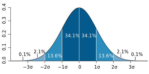
It is imprecise to compute the factorial of very large numbers, use the gaussian (normal) approximation instead
$$ p(x)=\frac{1}{\sqrt{2 \pi \sigma^2}} \exp \left( -\frac{(x-\mu)^2}{2 \sigma^2} \right) $$where $\sigma$ is the standard deviation and $\mu$ is the mean
This is nice because you can estimate the distribution in your head if you know the mean and standard deviation
In [26]:
gaus_prob_dist = []
pi = 3.1415926

for k in xrange(num_flips+1):
    var = expected_stdev**2
    num = math.exp(-(float(k)-expected_mean)**2/(2*var))
    denom = math.sqrt(2*pi*var)
    gaus_prob = num/denom
    gaus_prob_dist.append(gaus_prob)

plt.figure()
plt.plot(gaus_prob_dist, color='green', linewidth=4, linestyle='dashed')
plt.show()

In [27]:
## overlay the analytic distributions over the data
plt.figure()
plt.hist(head_counts, bins=range(num_flips), normed=True)
plt.plot(prob_dist, color='red', linewidth=4)
plt.plot(gaus_prob_dist, color='green', linewidth=4, linestyle='dashed')
plt.show()

How can you shift the distribution to be centered at higher or lower values, or have a broader/narrower peak?
In [27]: