MPI—Message Passing Interface
MPI is a library specification describing a parallel programming paradigm suitable for use on distributed-memory machines, such as modern supercomputers and distributed clusters.
In this lesson, we will review parallel programming concepts and introduce several useful MPI functions and concepts. We will work within this IPython notebook, which allows us to lay out our code, results, and commentary in the same interface. Feel free to open up a bash shell in the background if you prefer to look at and execute your code that way.
You may need to load Canopy on the UIUC EWS workstations first:
module load canopy
cd
ipython notebook
Background: Parallel Programming Paradigms
To better contextualize this, let us briefly review the basic parallel computing models in use today.
Computer Architecture
A classical computer processor receives instructions as sets of binary data from memory and uses these instructions (in assembly language) to manipulate data from memory in predictable ways. A processor works on a single piece of data at a time (although other data units may be waiting in the registers or cache) and executes a single thread, or sequential list, of commands on the data.
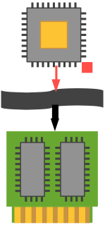
Thus we may say that a conventional desktop computer is SISD—Single Instruction, Single Data: a single program operates on a single data element sequentially, then exchanges it back into memory and retrieves a new datum. Any apparent multitasking is due to the operating system periodically switching the CPU's context from one thread to another. We will represent this scenario in the following graphic, which shows a single processor interacting via a bus (the wavy black band) with a collection of memory chips (which can be RAM, ROM, hard drives, etc.).
SIMD—Single Instruction, Multiple Data
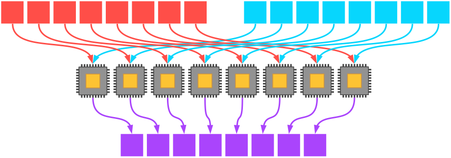
Springboarding off of SISD, perhaps the simplest way to think about a way of parallel programming is the SIMD model. In this model, multiple processing units operate simultaneously on multiple pieces of data in the same way.
Consider, for instance, the addition of two eight-element vectors. If we have eight processors available, then each processor can add two corresponding elements from the two vectors directly; the program then yields an efficiently added single eight-element vector afterwards (if we assume little to no overhead costs for the vectorization of the program).
(This, incidentally, was the major advantage of the first Cray supercomputers in the late 1970s: vectorization let them operate on many data elements simultaneously, thus achieving stupendous speedups.)
MIMD—Multiple Instruction, Multiple Data
Now it's not a major leap to think about using each of those processors to do something different to their assigned data element. It may not make much sense with vector addition, but when performing more complex operations like finite element differential equation solution or Monte Carlo random number integration, we often want a lot of plates spinning.
For MIMD to be effective, we need two different kinds of parallelism: data-level parallelism (can I segment my problem domain into complementary parts, whether in real space, time, or phase space?); and control-level parallelism (do I need different parts of my program to execute differently based on the data they have allotted to them?).
Imagine trying to calculate $\pi$ by throwing darts at a circle. We can count the number of darts that hit within the radius of the circle, $n_{\text{circle}}$, and compare that value with the ratio of all darts within a bounding square, $n_{\text{square}}$. (Physical simulation of this process is left as an exercise to the reader.) As we know the equations defining area, we can obtain $\pi$ trivially: $$\begin{array}{l} A_\text{circle} = \pi r^2 \\ A_\text{square} = 4 \pi r^2 \end{array} \implies r^2 = \frac{A_\text{square}}{4} = \frac{A_\text{circle}}{\pi} \implies \pi \approx 4 \frac{n_\text{circle}}{n_\text{square} + n_\text{circle}} \text{.}$$

It is apparent how this algorithm can benefit from parallelization: since any one dart is thrown independently of the others, we are not restricted from throwing a large number simultaneously. One possible algorithm could look like this:
initialize_memory
parallel {
    throw_dart
    total_darts = total_darts + 1
    count_my_darts_in_circle
}
add_all_darts_in_circle
add_all_darts
pi = 4 * darts_in_circle / total_darts
As you can see, in the parallel portion it doesn't matter to one processor what any other processor is doing. The only time we need all of the processors in sync is at the end of the parallel section where we add up all the darts thrown and that hit the circle. (We will return to this point later.)
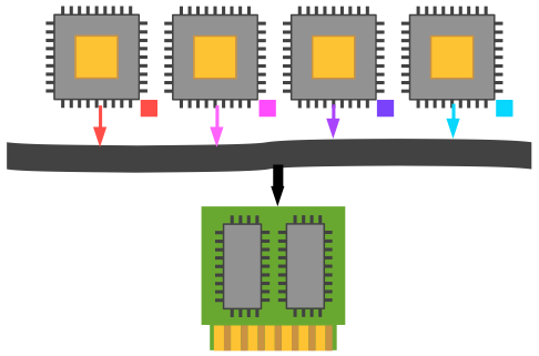
Let's take a look at the architecture of MIMD machines in a bit more detail now. The major division in MIMD programming is shared-memory v. distributed-memory systems.
Shared-Memory Systems
If the system architecture allows any processor to directly access any location in global memory space, then we refer to the machine as having a shared memory. This is convenient in practice for the programmer but can lead to inefficiencies in hardware and software library design. For instance, scaling beyond 32 or 64 processors has been a persistent problem for this architecture choice (contrast tens of thousands of processors for well-designed distributed-memory systems).
Examples of shared-memory parallelization specifications and libraries include OpenMP and OpenACC.
Addressing the dart-throwing problem above in the shared-memory paradigm is trivial, since each process can contribute its value from its unique memory location to the final result (a process known as reduction).
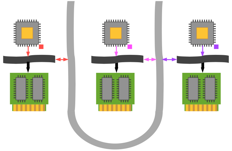
Distributed-Memory Systems
For distributed-memory MIMD architectures, every processor is alloted its own physical memory and has no knowledge of other processors' memory. This is the classic problem which MPI was designed to address: we now have to coördinate and communicate data across an internal network to allow these processors to work effectively together.
The dart-throwing example from before is now nontrivial, but completely scalable (subject to communication overhead). Every processor is independent and can calculate for one or many darts thrown. However, some sort of reduction must be performed to obtain a final coherent result for the number of darts within the circle (the total number should be known a priori from the number of processes, presumably). The pseudocode in this case looks more like this:
initialize_memory
parallel {
    throw_dart
    total_darts = total_darts + 1
    count_my_darts_in_circle
}
darts_in_circle = reduction_over_all_processors_of_darts_in_their_circles
add_all_darts
pi = 4 * darts_in_circle / total_darts
We will shortly examine this case as implemented in MPI.
MPI Basics
Hello World
The classical example for any new programming language or library is to construct a nontrivial "Hello World!" program. In the following code (./src/mpi-mwe/c/hello_world_mpi.c), we will see the basic elements of any MPI program, including preliminary setup, branching into several processes, and cleanup when program execution is about to cease. (No message passing occurs in this example.)
%%file hello_world_mpi.c
#include <stdio.h>
#include <mpi.h>

int main(int argc, char *argv[]) {
    int     rank_id, ierr, num_ranks;
    double  start_time, wall_time;

    printf("C MPI minimal working example\n");

    ierr = MPI_Init(&argc, &argv);
    start_time = MPI_Wtime();
    ierr = MPI_Comm_size(MPI_COMM_WORLD, &num_ranks);
    ierr = MPI_Comm_rank(MPI_COMM_WORLD, &rank_id);

    if (rank_id == 0) {
        printf("Number of available processors = %d.\n", num_ranks);
    }
    printf("\tProcess number %d branching off.\n", rank_id);

    wall_time = MPI_Wtime() - start_time;

    if (rank_id == 0) {
        printf("Elapsed wallclock time = %8.6fs.\n", wall_time);
    }

    MPI_Finalize();
    return 0;
}
Let’s compile and execute this program before commenting on its contents. In order to link the program properly, there are a number of MPI libraries and include files which need to be specified. Fortunately, a convenient wrapper around your preferred C/C++/Fortran compiler has been provided: in this case, mpicc. To see what the wrapper is doing behind the scenes, use the -show option:
$ mpicc -show
clang -I/usr/local/Cellar/open-mpi/1.8.1/include
      -L/usr/local/opt/libevent/lib
      -L/usr/local/Cellar/open-mpi/1.8.1/lib -lmpi
We can thus compile and execute the above example by simply entering,
$ mpicc -o hello_world_mpi hello_world_mpi.c
$ ./hello_world_mpi C MPI minimal working example Number of available processors = 1. Process number 0 branching off. Elapsed wallclock time = 0.000270s.
!mpicc -o hello_world_mpi hello_world_mpi.c
!./hello_world_mpi
Now, that's not right, is it? I have a number of processors on my modern machine, so why didn't this use them? In the case of MPI, it is necessary to use the script mpiexec which sets up the copies in parallel and coördinates message passing.
$ mpiexec ./hello_world_mpi
C MPI minimal working example
C MPI minimal working example
C MPI minimal working example
C MPI minimal working example
    Process number 1 branching off.
Number of available processors = 4.
    Process number 0 branching off.
Elapsed wallclock time = 0.000021s.
    Process number 2 branching off.
    Process number 3 branching off.
!mpiexec ./hello_world_mpi
(Note the race conditions apparent here: with input and output, unless you explicitly control access and make all of the threads take turns, the output order is unpredictable.)
Okay, let's step back and analyze the program now, noting the following points:
- MPI functions pass values by reference.
- MPI functions do not return the value of the variable they modify, but rather an error code. The modified value is in the referenced variable.
- A universal communicator,
MPI_COMM_WORLD, is defined to permit communication with all processes. (Subsets of this may be defined as desired.) MPI_InitandMPI_Finalizemust be called to initialize and terminate the message-passing environment.
Exercise
- Run the "Hello World" script with 1, 2, 4, 8, and 16 processes. See if the time required varies significantly. Try this with other numbers as well: 3, 7, etc.
!mpiexec -np 1 ./hello_world_mpi
Message Passing: MPI_Send, MPI_Recv
At the highest level, an MPI implementation supports the parallel execution of a number of copies of a program which can intercommunicate with each other across an equal number of processors. Internode and intranode communications are implicitly handled by the operating system, interconnect, and MPI libraries.
The fundamental pair of actions for a processor using MPI is sending and receiving messages. (This is also known as point-to-point communication.) A number of more complex actions, such as the partitioning of data or collection of calculated results, are built from these point-to-point communications. Finally, more advanced features exist to customize the processor topology, operations, and process management.
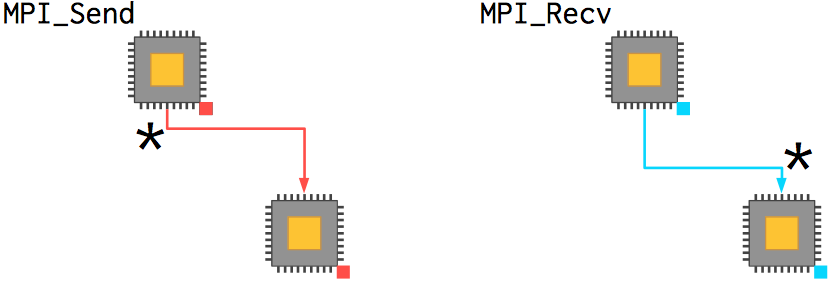
Send and receive actions are always paired with each other. There are a number of flavors, but let's start with the basic two: MPI_Send and MPI_Recv. The function prototypes are:
int MPI_Send(
    void*        message,          // Pointer to data to send
    int          count,            // Number of data values to send
    MPI_Datatype datatype,         // Type of data (e.g. MPI_INT)
    int          destination_rank, // Rank of process to receive message
    int          tag,              // Identifies message type
    MPI_Comm     comm              // Use MPI_COMM_WORLD
)

int MPI_Recv(
    void*        message,     // Points to location in memory where
                              //     received message is to be stored.
    int          count,       // MAX number of data values to accept
    MPI_Datatype datatype     // Type of data (e.g. MPI_INT)
    int          source_rank, // Rank of process to receive from
                              //    (Use MPI_ANY_SOURCE to accept
                              //     from any sender)
    int          tag,         // Type of message to receive
                              //    (Use MPI_ANY_TAG to accept any type)
    MPI_Comm     comm,        // Use MPI_COMM_WORLD
    MPI_Status*  status       // To receive info about the message
)
There's a lot of information there, and none of it optional (if you want to hide it, use a language and package such as Python and MPI4Py). Let's unpack the arguments a little more with a trivial example that implements the previous dart-throwing example.
%%file darts_pi.c
#include <math.h>
#include <stdio.h>
#include <stdlib.h>
#include <time.h>
#include <mpi.h>

#define N 100000
#define R 1

double uniform_rng() { return (double)rand() / (double)RAND_MAX; } // Not great but not the point of this exercise.

int main(int argc, char *argv[]) {
    int     rank_id, ierr, num_ranks;
    MPI_Status status;

    ierr = MPI_Init(&argc, &argv);
    ierr = MPI_Comm_size(MPI_COMM_WORLD, &num_ranks);
    ierr = MPI_Comm_rank(MPI_COMM_WORLD, &rank_id);
    srand(time(NULL) + rank_id);

    //  Calculate some number of darts thrown into the circle.
    int n_circle = 0;
    double x, y;
    for (int t = 0; t < N; t++) {
        x = uniform_rng();
        y = uniform_rng();
        if (x*x + y*y < (double)R*R) n_circle++;
    }

    //  If this is the first process, then gather everyone's data.  Otherwise, send it to the first process.
    int total_circle[num_ranks]; // C99 Variable Length Arrays; compile with `-std=c99` or else use `malloc`.
    if (rank_id == 0) {
        total_circle[0] = n_circle;
        for (int i = 1; i < num_ranks; i++) {
            ierr = MPI_Recv(&total_circle[i], 1, MPI_INT, i, MPI_ANY_TAG, MPI_COMM_WORLD, &status);
            //printf ("\t%d: recv %d from %d\n", rank_id, total_circle[i], i);
        }
    } else {
        ierr = MPI_Send(&n_circle, 1, MPI_INT, 0, 1, MPI_COMM_WORLD);
        //printf ("\t%d: send %d to %d\n", rank_id, n_circle, 0);
    }

    //  Now sum over the data and calculate the approximation of pi.
    int total = 0;
    if (rank_id == 0) {
        for (int i = 0; i < num_ranks; i++) {
            total += total_circle[i];
        }
        printf("With %d trials, the resulting approximation to pi = %f.\n", num_ranks*N, 4.0*(double)total/((double)N*(double)num_ranks));
    }

    MPI_Finalize();
    return 0;
}
Compile and execute this code in the shell:
$ mpicc -std=c99 -o darts_pi darts_pi.c
$ mpiexec -n 4 ./darts_pi With 400000 trials, the resulting approximation to pi = 3.137710. Elapsed wallclock time = 0.002829s.
A few remarks:
- We know this algorithm is inefficient: 400,000 trials for 2 digits of accuracy is absurd! Compare a series solution, which should give you that in a handful of terms.
- I don't do a great job of calculating the random values as floating-point values, just dividing by the maximum possible integer value from
stdlib.h. (This example is doubly dangerous in that it assumes that the default C random number library is thread safe! It is not!—more on that in the OpenMP lesson.) - Note how we are accessing the respective elements of the array
total_circlein theMPI_Recvclause. - We limit the efficiency by receiving the messages in order.
# To run this code from within the notebook.
!mpicc -std=c99 -o darts_pi darts_pi.c
!mpiexec -n 4 ./darts_pi
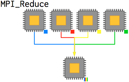
Collective Operations: MPI_Reduce
We can render this function much more readable and less error-prone by using the convenience function MPI_Reduce, which achieves the same effective outcome as the prior code without the explicit message management. Reduction takes a series of values from each processor, applies some operation to them, and then places the result on the root process (which doesn't have to be 0, although it often is).
int MPI_Reduce(
    void*        value,      // Input value from this process
    void*        answer,     // Result -- on root process only
    int          count,      // Number of values -- usually 1
    MPI_Datatype datatype,   // Type of data (e.g. MPI_INT)
    MPI_Op       operation,  // What to do (e.g. MPI_SUM)
    int          root,       // Process that receives the answer
    MPI_Comm     comm        // Use MPI_COMM_WORLD
)
In the context of our prior code, we can convert the code segment as follows:
%%file darts_pi.c
#include <math.h>
#include <stdio.h>
#include <stdlib.h>
#include <time.h>
#include <mpi.h>

#define N 100000
#define R 1

double uniform_rng() { return (double)rand() / (double)RAND_MAX; } // Not good but not the point of this exercise.

int main(int argc, char *argv[]) {
    int     rank_id, ierr, num_ranks;
    MPI_Status status;

    ierr = MPI_Init(&argc, &argv);
    ierr = MPI_Comm_size(MPI_COMM_WORLD, &num_ranks);
    ierr = MPI_Comm_rank(MPI_COMM_WORLD, &rank_id);
    srand(time(NULL) + rank_id);

    //  Calculate some number of darts thrown into the circle.
    int n_circle = 0;
    double x, y;
    for (int t = 0; t < N; t++) {
        x = uniform_rng();
        y = uniform_rng();
        if (x*x + y*y < (double)R*R) n_circle++;
    }

    //  Reduce by summation over all data and output the result.
    int total;
    ierr = MPI_Reduce(&n_circle, &total, 1, MPI_INT, MPI_SUM, 0, MPI_COMM_WORLD);
    if (rank_id == 0) {
        printf("With %d trials, the resulting approximation to pi = %f.\n", num_ranks*N, 4.0*(double)total/((double)N*(double)num_ranks));
    }

    MPI_Finalize();
    return 0;
}
# To run this code from within the notebook.
!mpicc -std=c99 -o darts_pi darts_pi.c
!mpiexec -n 4 ./darts_pi
That reduces ten significant lines of code, two for loops, $N_\text{processor}$ MPI function calls, and an array allocation to a single MPI function call. Not bad. This is typical, I find, of numerical codes: well-written MPI code in a few key locations covers the bulk of your communication needs, and you rarely need to explicitly pass messages or manage processes dynamically.
A Finite Difference Example
Let's look through an integrated example which will introduce a few new functions and give you a feel for how MPI operates in a larger code base. We will utilize the finite difference method to solve Poisson's equation for an electrostatic potential: $${\nabla}^2 \varphi = -\frac{\rho_f}{\varepsilon}$$ where $\rho_f$ are the (known) positions of charges; $\varepsilon$ is the permittivity of the material; and $\varphi$ is the resultant scalar electric potential field.
We use a second-order central difference scheme in the discretization of the differential equation in space and take an initial guess which will require iteration to obtain a steady-state solution. The resulting equation for an arbitrary location in the $(x, y)$ grid (assuming uniform discretization) subject to a set of discrete point charges $\sum \rho_f$ is: $$\frac{\varphi_{i+1,j}-2\varphi_{i,j}+\varphi_{i-1,j}}{\delta^2} + \frac{\varphi_{i,j+1}-2\varphi_{i,j}+\varphi_{i,j-1}}{\delta^2} = \frac{\sum \rho_f}{\varepsilon} \implies$$ $$\varphi_{i,j} = \frac{1}{4} \left(\varphi_{i+1,j}+\varphi_{i-1,j}+\varphi_{i,j+1}+\varphi_{i,j-1}\right) - \frac{\Delta^2}{4} \left(\frac{\sum \rho_f}{\varepsilon}\right) \text{.}$$ (As the discretization does not subject grid locations to nonlocal influences, it is necessary for the grid locations next to the point charges to propagate that information outward as the iteration proceeds towards a solution.)
For some known distribution of charges, we can construct a matrix equation and solve it appropriately either by hand-coding an algorithm or by using a library such as GNU Scientific Library. In this case, to keep things fairly explicit, we won't write a matrix explicitly and will instead solve each equation in a for loop.
Serial Code
One of the odd things we need to consider is that because we are using point charges our grid has to overlap with them directly. (This isn't as much of a problem with distributions.) So we'll just start with a handful of point charges for now, with the boundaries from $(-1,-1)$ to $(1,1)$ set to zero.
%%file fd_charge.c
//  This is a serial version of the code for reference.
#include <math.h>
#include <stdio.h>
#include <stdlib.h>
#include <string.h> //for memcpy()
#include <time.h>

#define BOUNDS 1.0

double uniform_rng() { return (double)rand() / (double)RAND_MAX; } // Not good but not the point of this exercise.
struct point_t { int x, y; double mag; };

int main(int argc, char *argv[]) {
    int N = 10;
    if (argc > 1) N = atoi(argv[1]);
    int size = N % 2 == 0 ? N : N+1;  // ensure odd N
    int iter = 10;
    if (argc > 2) iter = atoi(argv[2]);
    int out_step = 1000;
    if (argc > 3) out_step = atoi(argv[3]);
    double eps = 8.8541878176e-12; // permittivity of the material
    srand(time(NULL));

    //  Initialize the grid with an initial guess of zeros as well as the coordinates.
    double phi[size][size];    // C99 Variable Length Arrays; compile with `-std=c99` or else use `malloc`.
    double oldphi[size][size];
    double x[size],
           y[size];
    double dx = (2*BOUNDS)/size,
           dy = dx;
    for (int i = 0; i < size; i++) {
        x[i] = (double)i*dx - BOUNDS;
        for (int j = 0; j < size; j++) {
            if (i == 0) y[j] = (double)j*dy - BOUNDS;
            phi[i][j] = 0.0;
        }
    }
    //  Set up a few random points and magnitudes for the electrostatics problem.
    int K = 20;
    struct point_t pt_srcs[K];
    for (int k = 0; k < K; k++) {
        pt_srcs[k].x   = (int)(uniform_rng() * N);
        pt_srcs[k].y   = (int)(uniform_rng() * N);
        pt_srcs[k].mag = uniform_rng() * 2.0 - 1.0;
        printf("(%f, %f) @ %f\n", x[pt_srcs[k].x], y[pt_srcs[k].y], pt_srcs[k].mag);
    }

    //  Iterate forward.
    int    n_steps = 0;        // total number of steps iterated
    double inveps = 1.0 / eps; // saves a division every iteration over the square loop
    double pt_src = 0.0;       // accumulator for whether a point source is located at a specific (i,j) index site
    while (n_steps < iter) {
        memcpy(oldphi, phi, size*size);
        for (int i = 0; i < size; i++) {
            for (int j = 0; j < size; j++) {
                //  Calculate point source contributions.
                pt_src = 0;
                for (int k = 0; k < K; k++) {
                    pt_src = pt_src + ((pt_srcs[k].x == i && pt_srcs[k].y == j) ? pt_srcs[k].mag : 0.0);
                }
                phi[i][j] = 0.25*dx*dx * pt_src * inveps
                          + 0.25*(i == 0      ? 0.0 : phi[i-1][j])
                          + 0.25*(i == size-1 ? 0.0 : phi[i+1][j])
                          + 0.25*(j == 0      ? 0.0 : phi[i][j-1])
                          + 0.25*(j == size-1 ? 0.0 : phi[i][j+1]);
            }
        }
        if (n_steps % out_step == 0) {
            printf("Iteration #%d:\n", n_steps);
            printf("\tphi(%f, %f) = %24.20f\n", x[(int)(0.5*N-1)], y[(int)(0.25*N+1)], phi[(int)(0.5*N-1)][(int)(0.25*N+1)]);
        }
        n_steps++;
    }

    //  Write the final condition out to disk and terminate.
    printf("Terminated after %d steps.\n", n_steps);

    FILE* f;
    f = fopen("./data.txt", "w"); // wb -write binary
    if (f != NULL) {
        for (int i = 0; i < size; i++) {
            for (int j = 0; j < size; j++) {
                fprintf(f, "%f\t", phi[i][j]);
            }
            fprintf(f, "\n");
        }
        fclose(f);
    } else {
        //failed to create the file
    }

    return 0;
}
!mpicc -std=c99 -o fd_charge fd_charge.c
!./fd_charge 200 80000 1000
# Use Python to visualize the result quickly.
import numpy as np
import matplotlib as mpl
import matplotlib.pyplot as plt
from matplotlib import cm
%matplotlib inline
#mpl.rcParams['figure.figsize']=[20,20]

data = np.loadtxt('./data.txt')
grdt = np.gradient(data);
mx = 10**np.floor(np.log10(data.max()))

fig, axes = plt.subplots(nrows=1, ncols=2, figsize=(20,20))
axes[0].imshow(data, cmap=cm.seismic, vmin=-mx, vmax=mx, extent=[-1,1,-1,1])
axes[1].imshow(data, cmap=cm.seismic, vmin=-mx, vmax=mx)
#axes[1].quiver(grdt[0].T, grdt[1].T, scale=5e8) #only good for N < 50
axes[1].contour(data, cmap=cm.bwr, vmin=-mx, vmax=mx, levels=np.arange(-mx,mx+1,(2*mx)/1e2))
fig.show()
So for a quick and dirty job (and no validation or verification of the numerics), that serial code will do. But you can already notice significant slowdown towards convergence even at 400×400 resolution (0.025 length units). To handle bigger problems, it will be necessary to parallelize.
Parallel Code
We will restrict the domain decomposition to square numbers of processes for the sake of pedagogy, although you likely wouldn't be this restrictive in a real code. Each processor will be responsible for calculating the electrostatics on its segment of the domain, and will not actually have access to the values calculated by the other processes unless they are explicitly communicated.
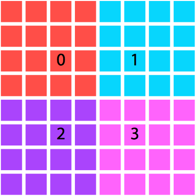 One decomposition of a domain by area and processor. |
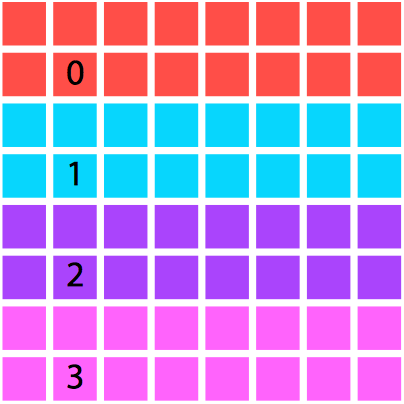 An alternative. Although we opted for the left-hand setting |
Why would we need to communicate any values? Well, in this case, parallelization is nontrivial: the finite difference algorithm is nearest-neighbor based, so with a spatial decomposition of the domain we will still need to communicate boundary cells to neighboring processes. Thus we will require ghost cells, which refer to data which are not located on this processor natively but are retrieved and used in calculations on the boundary of the local domain.
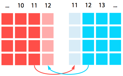
We can set these up either by having separate arrays for the ghost cells (which leads to clean messaging but messy numerical code) or having integrated arrays in the main phi array (which leads to nasty messaging code but nicer numerics). We will use clean messaging to clarify the message passing aspect at the cost of obfuscating the numerics a bit with nested ternary cases.
%%file fd_charge.c
//  This is a parallel version of the code.
#include <math.h>
#include <stdio.h>
#include <stdlib.h>
#include <string.h> //for memcpy()
#include <time.h>
#include <mpi.h>

#define BOUNDS 1.0

double uniform_rng() { return (double)rand() / (double)RAND_MAX; } // Not good but not the point of this exercise.
struct point_t { int x, y; double mag; };

int main(int argc, char *argv[]) {
    int size = 10;
    if (argc > 1) size = atoi(argv[1]);
    int iter = 10;
    if (argc > 2) iter = atoi(argv[2]);
    int out_step = 1000;
    if (argc > 3) out_step = atoi(argv[3]);
    double eps = 8.8541878176e-12; // permittivity of the material

    int     rank_id, ierr, num_ranks;
    MPI_Status  status;
    MPI_Request request;

    ierr = MPI_Init(&argc, &argv);
    ierr = MPI_Comm_size(MPI_COMM_WORLD, &num_ranks);
    ierr = MPI_Comm_rank(MPI_COMM_WORLD, &rank_id);
    srand(time(NULL) + rank_id);

    //  We will restrict partitions of the domain (and thus processes) to square numbers for the sake of pedagogy.
    //  Not fast, not elegant, but we only do it once.
    if (abs(sqrt((float)num_ranks)-(int)sqrt((float)num_ranks)) > 1e-6) {
        printf("Expected square number for number of processes; actual number %f.\n", (float)abs((float)sqrt((float)num_ranks)));
        MPI_Abort(MPI_COMM_WORLD, MPI_ERR_OTHER);
        return 0;
    }

    //  Calculate the processor grid preparatory to the domain partition.  We'll make the assignment into a
    //  sqrt(N) x sqrt(N) array.  This allows easy determination of neighboring processes.
    int base = (int)abs(sqrt(num_ranks));
    int nbr_l = rank_id % base - 1 >= 0   ? rank_id - 1    : -1; //printf("%d: nbr_l = %d\n", rank_id, nbr_l);
    int nbr_r = rank_id % base + 1 < base ? rank_id + 1    : -1; //printf("%d: nbr_r = %d\n", rank_id, nbr_r);
    int nbr_t = rank_id + base < num_ranks? rank_id + base : -1; //printf("%d: nbr_t = %d\n", rank_id, nbr_t);
    int nbr_b = rank_id - base >= 0       ? rank_id - base : -1; //printf("%d: nbr_b = %d\n", rank_id, nbr_b);

    //  Initialize the _local_ grid with an initial guess of zeros as well as the coordinates.  We will keep each
    //  local domain the same size as the original domain, 2x2 in coordinates, and just translate them to make a
    //  larger domain---in this case, adding processes increases the domain size rather than the mesh resolution.
    double phi[size][size];    // C99 Variable Length Arrays; compile with `-std=c99` or else use `malloc`.
    double oldphi[size][size];
    double x[size],
           y[size];
    double dx = (2*BOUNDS)/size,
           dy = dx;
    double base_x = 2*BOUNDS*(rank_id % base) - BOUNDS*base,
           base_y = 2*BOUNDS*(rank_id - (rank_id % base)) / base - BOUNDS*base;
    for (int i = 0; i < size; i++) {
        x[i] = (double)i*dx + base_x;
        for (int j = 0; j < size; j++) {
            if (i == 0) y[j] = (double)j*dy + base_y;
            phi[i][j] = 0.0;
        }
    }
    double phi_l_in[size], // ghost cell messaging arrays
           phi_r_in[size],
           phi_t_in[size],
           phi_b_in[size],
           phi_l_out[size],
           phi_r_out[size],
           phi_t_out[size],
           phi_b_out[size];
    for (int i = 0; i < size; i++) {
        phi_l_in[i]  = 0.0;
        phi_r_in[i]  = 0.0;
        phi_t_in[i]  = 0.0;
        phi_b_in[i]  = 0.0;
    }
    //printf("%d: (%f,%f)-(%f,%f)\n", rank_id, base_x, base_y, x[size-1], y[size-1]);

    //  Set up a few random points and magnitudes for the electrostatics problem.
    int K = 80;
    struct point_t pt_srcs[K];
    for (int k = 0; k < K; k++) {
        (uniform_rng()); // proof that the RNG is bad:  without this the first number is the same on every thread.
        int x_rn = (int)(uniform_rng() * size);
        int y_rn = (int)(uniform_rng() * size);
        pt_srcs[k].x   = x_rn;
        pt_srcs[k].y   = y_rn;
        pt_srcs[k].mag = uniform_rng() * 2.0 - 1.0;
        //printf("%d: [%d, %d] (%f, %f) @ %f\n", rank_id, x_rn, y_rn, x[pt_srcs[k].x], y[pt_srcs[k].y], pt_srcs[k].mag);
    }

    //  Iterate forward.
    int    n_steps = 0;        // total number of steps iterated
    double inveps = 1.0 / eps; // saves a division every iteration over the square loop
    double pt_src = 0.0;       // accumulator for whether a point source is located at a specific (i,j) index site
    while (n_steps < iter) {
        memcpy(oldphi, phi, size*size); // Back up the old matrix for residual comparison, if desired.
        //  Propagate the matrix equation forward towards a solution.
        for (int i = 0; i < size; i++) {
            for (int j = 0; j < size; j++) {
                //  Calculate point source contributions.
                pt_src = 0;
                for (int k = 0; k < K; k++) {
                    pt_src = pt_src + ((pt_srcs[k].x == i && pt_srcs[k].y == j) ? pt_srcs[k].mag : 0.0);
                }
                phi[i][j] = 0.25*dx*dx * pt_src * inveps
                          + 0.25*(i == 0      ? (nbr_l < 0 ? 0.0 : phi_l_in[j]) : phi[i-1][j])
                          + 0.25*(i == size-1 ? (nbr_r < 0 ? 0.0 : phi_r_in[j]) : phi[i+1][j])
                          + 0.25*(j == 0      ? (nbr_b < 0 ? 0.0 : phi_b_in[i]) : phi[i][j-1])
                          + 0.25*(j == size-1 ? (nbr_t < 0 ? 0.0 : phi_t_in[i]) : phi[i][j+1]);
            }
        }

        //  Communicate the border cell information to neighboring processes.  We will alternate odd and even processes,
        //  although there are more sophisticated ways to do this with nonblocking message passing.  Why do we alternate?
        for (int i = 0; i < size; i++) {
            phi_l_out[i] = phi[0][i];
            phi_r_out[i] = phi[size-1][i];
            phi_t_out[i] = phi[i][size-1];
            phi_b_out[i] = phi[i][0];
        }
        //    Pass data left.
        if (nbr_l >= 0) MPI_Isend(phi_l_out, size, MPI_DOUBLE, nbr_l, 0,           MPI_COMM_WORLD, &request);
        if (nbr_r >= 0) MPI_Irecv(phi_r_in,  size, MPI_DOUBLE, nbr_r, MPI_ANY_TAG, MPI_COMM_WORLD, &request);

        //    Pass data right.
        if (nbr_r >= 0) MPI_Isend(phi_r_out, size, MPI_DOUBLE, nbr_r, 0,           MPI_COMM_WORLD, &request);
        if (nbr_l >= 0) MPI_Irecv(phi_l_in,  size, MPI_DOUBLE, nbr_l, MPI_ANY_TAG, MPI_COMM_WORLD, &request);

        //    Pass data up.
        if (nbr_t >= 0) MPI_Isend(phi_t_out, size, MPI_DOUBLE, nbr_t, 0,           MPI_COMM_WORLD, &request);
        if (nbr_b >= 0) MPI_Irecv(phi_b_in,  size, MPI_DOUBLE, nbr_b, MPI_ANY_TAG, MPI_COMM_WORLD, &request);

        //    Pass data down.
        if (nbr_b >= 0) MPI_Isend(phi_b_out, size, MPI_DOUBLE, nbr_b, 0,           MPI_COMM_WORLD, &request);
        if (nbr_t >= 0) MPI_Irecv(phi_t_in,  size, MPI_DOUBLE, nbr_t, MPI_ANY_TAG, MPI_COMM_WORLD, &request);
        MPI_Barrier(MPI_COMM_WORLD);

        //  Output information periodically.
        if (rank_id == 0 && n_steps % out_step == 0) {
            printf("Iteration #%d:\n", n_steps);
            printf("\tphi(%6.3f, %6.3f) = %24.20f\n", x[(int)(0.5*size-1)], y[(int)(0.25*size+1)], phi[(int)(0.5*size-1)][(int)(0.25*size+1)]);
        }
        n_steps++;
    }
    if (rank_id == 0) {
        printf("Terminated after %d steps.\n", n_steps);
        printf("\tphi(%6.3f, %6.3f) = %24.20f\n", x[(int)(0.5*size-1)], y[(int)(0.25*size+1)], phi[(int)(0.5*size-1)][(int)(0.25*size+1)]);
    }

    //  Write the final condition out to disk and terminate.
    //  Parallel I/O, while supported by MPI, is a whole other ball game and we won't go into here.
    //  Thus we will gather all of the data to process rank 0 and output it from there.
    double phi_all[size*base*size*base];
    //  This version of the code ^ incorrectly orders the processor output.  We actually have to transpose each process's
    //  data into a column-major format to get everything aligned properly.
    double phi_temp[size][size];
    for (int i = 0; i < size; i++) {
        for (int j = 0; j < size; j++) {
            phi_temp[j][i] = phi[i][j];
        }
    }
    MPI_Gather(&phi_temp[0][0], size*size, MPI_DOUBLE, &phi_all[0], size*size, MPI_DOUBLE, 0, MPI_COMM_WORLD);
    //  At this point, the data are in the right array, but have an odd stride and relative order.  We'll fix that now.
    double phi_new[size*base][size*base];
    int offset_x, offset_y;
    for (int p = 0; p < base*base; p++) {     // source process for data
        offset_x = (p-p%base)/base;
        offset_y = (p%base);
        for (int i = 0; i < size; i++) {      // x-index of process data
            for (int j = 0; j < size; j++) {  // y-index of process data
                phi_new[offset_y*size+j][offset_x*size+i] = phi_all[p*size*size+i*size+j];
            }
        }
    }

    if (rank_id == 0) {
        FILE* f;
        char filename[16];
        f = fopen("data.txt", "w"); // wb -write binary
        if (f != NULL) {
            for (int i = 0; i < base*size; i++) {
                for (int j = 0; j < base*size; j++) {
                    fprintf(f, "%f\t", phi_new[i][j]);
                }
                fprintf(f, "\n");
            }
            fclose(f);
        } else {
            //failed to create the file
        }
    }

    MPI_Finalize();
    return 0;
}
!mpicc -std=c99 -o fd_charge fd_charge.c
!mpiexec -np 9 ./fd_charge 100 100001 5000
# Use Python to visualize the result quickly.
import numpy as np
import matplotlib as mpl
import matplotlib.pyplot as plt
from matplotlib import cm
%matplotlib inline

data = np.loadtxt('./data.txt')
mx = 10**np.floor(np.log10(data.max()))

fig, axes = plt.subplots(nrows=1, ncols=1, figsize=(16,16))
axes.imshow(data, cmap=cm.seismic, vmin=-mx, vmax=mx)
fig.show()

fig, axes = plt.subplots(nrows=1, ncols=1, figsize=(16,16))
axes.contour(data[::-1,:], cmap=cm.bwr, vmin=-mx, vmax=mx, levels=np.arange(-mx,mx+1,(2*mx)/1e2))
fig.show()
What happens if I neglect to include the following conditional around the file output?
if (rank_id == 0) { ... }
Domains naturally do not overlap in this case:
0: (-2.00,-2.00)-(-0.01,-0.01)
1: ( 0.00,-2.00)-( 1.99,-0.01)
2: (-2.00, 0.00)-(-0.01, 1.99)
3: ( 0.00, 0.00)-( 1.99, 1.99)
Message Passing: MPI_Isend, MPI_Irecv
The vanilla MPI send and receive operations are blocking, meaning that when you send a message the process waits at that point until an acknowledgment of receipt is sent by the receiving process. As you can imagine, this both slows down your code and makes even simple messaging schemes cumbersome (what happens if you tell every process to send at the same time and receive at the next function call?). In order to prevent this kind of deadlock, we use nonblocking communications, which do not block execution—they just fire their message into the ether and proceed ahead.
As before, there are a lot of variants, but the basic two are MPI_Isend and MPI_Irecv.
int MPI_Isend(
    void*        message,          // Pointer to data to send
    int          count,            // Number of data values to send
    MPI_Datatype datatype,         // Type of data (e.g. MPI_INT)
    int          destination_rank, // Rank of process to receive message
    int          tag,              // Identifies message type
    MPI_Comm     comm,             // Use MPI_COMM_WORLD
    MPI_Request* request           // To query about the status of the message
)

int MPI_Irecv(
    void*        message,     // Points to location in memory where
                              //     received message is to be stored.
    int          count,       // MAX number of data values to accept
    MPI_Datatype datatype     // Type of data (e.g. MPI_INT)
    int          source_rank, // Rank of process to receive from
                              //    (Use MPI_ANY_SOURCE to accept
                              //     from any sender)
    int          tag,         // Type of message to receive
                              //    (Use MPI_ANY_TAG to accept any type)
    MPI_Comm     comm,        // Use MPI_COMM_WORLD
    MPI_Request* request      // To query about the status of the message
)
There's a lot of information there, and none of it optional. Let's unpack the arguments a little more with a trivial example that implements the previous dart-throwing example.
Collective Operations: MPI_Barrier, MPI_Gather
Now, with nonblocking operations we can easily run into a situation where we need to know that a certain message has already been received in order to coherently progress: the array needs to be updated, whatever. In that case, MPI_Barrier defines a point at which all processes will wait until they are synchronized with each other again. They slow code down, however, and so they should be used sparingly.
int MPI_Barrier(
    MPI_Comm     comm        // Use MPI_COMM_WORLD
)
Exercise
What is the difference in the following two code snippets?
// Pass data left. if (nbr_l >= 0) MPI_Isend(phi_l_out, size, MPI_DOUBLE, nbr_l, 0, MPI_COMM_WORLD, &request); if (nbr_r >= 0) MPI_Irecv(phi_r_in, size, MPI_DOUBLE, nbr_r, MPI_ANY_TAG, MPI_COMM_WORLD, &request); if (nbr_l >= 0 && n_steps == 1000) printf("%d: %d sending left %f to %d\n", n_steps, rank_id, phi_l_out[5], nbr_l); if (nbr_r >= 0 && n_steps == 1000) printf("%d: %d recving right %f of %d\n", n_steps, rank_id, phi_r_in[5], nbr_r); MPI_Barrier(MPI_COMM_WORLD);
// Pass data left. if (nbr_l >= 0) MPI_Isend(phi_l_out, size, MPI_DOUBLE, nbr_l, 0, MPI_COMM_WORLD, &request); if (nbr_r >= 0) MPI_Irecv(phi_r_in, size, MPI_DOUBLE, nbr_r, MPI_ANY_TAG, MPI_COMM_WORLD, &request); MPI_Barrier(MPI_COMM_WORLD); if (nbr_l >= 0 && n_steps == 1000) printf("%d: %d sending left %f to %d\n", n_steps, rank_id, phi_l_out[5], nbr_l); if (nbr_r >= 0 && n_steps == 1000) printf("%d: %d recving right %f of %d\n", n_steps, rank_id, phi_r_in[5], nbr_r);
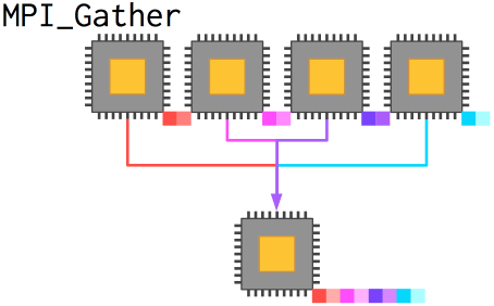
MPI_Gather
Previously, we examined the function MPI_Reduce, which took data from every process, transformed them by some operation like addition or multiplication, and placed the result in a variable on root. In the case above, we needed to gather data from every process without transforming the data or collapsing it from an array to a single value.
MPI_Gather takes arrays from every process and combines them (by rank) into a new array on root. The new array, as we saw above, is ordered by rank, meaning that if a different topology is in use you have to correct the data (which we did).
int MPI_Gather(
    void*        sendbuf,    // Starting address of send buffer
    int          sendcnt,    // Number of elements in send buffer
    MPI_Datatype datatype,   // Type of data (e.g. MPI_INT)
    void*        recvbuf,    // Starting address of receive buffer
    int          recvcnt,    // Number of elements for any single receive
    MPI_Datatype recvtype,   // Type of data (e.g. MPI_INT)
    int          root,       // Process that receives the answer
    MPI_Comm     comm        // Use MPI_COMM_WORLD
)
In this case, MPI is a lot more work, but you gain the capability of scaling to a reasonably large number of processors.
Scaling
Scaling refers to how efficiently your code retains performance as both the problem size $N$ and the number of processes $P$ increase. It is typically divided into weak and strong scaling.
Strong Scaling: How does the performance behave as the number of processors $P$ increases for a fixed total problem size $N$?
This is what most people think of as scaling, and describes the overall performance of a code as a problem is subdivided into smaller and smaller pieces between processes. To test this, select a problem size suitable to scaling to a large number of processes (for instance, divisible by 64), and simply call larger and larger jobs while outputting timing information.
Weak Scaling: How does the performance behave as the number of processors $P$ varies with each processor handling a fixed process size $N_P = N/P = \text{const}$?
In this case (which is most appropriate for $O(N)$ algorithms but can be used for any system), we observe more about the relative overhead incurred by including additional machines in the problem solution. Weak scaling can be tested in a straightforward manner by keeping track of the pieces of the puzzle each process is responsible for. With strongly decomposable systems, like molecular dynamics or PDE solution on meshes, weak scaling can be revealing. However, in my experience there are many types of problems for which solving for $N$ and solving for $N+1$ are radically different problems, such as in density functional theory where the addition of an electron means the solution of a fundamentally different physical system.
(ref)
Memory and C99 Variable-Length Arrays
Are the following two segments of code equivalent in C99?
Snippet 1
int m = 5, n = 10, p = 7;
double array[m][n][p];
Snippet 2
double ***array;
array = (double***) malloc(m*sizeof(double**));
for (i = 0; i < m; i++) {
   array[i] = (double**) malloc(n*sizeof(double*));
   for (j = 0; j < n; j++) {
       array[i][j] = (double*) malloc(p*sizeof(double));
   }
}
They aren't_—but you may not be sure why. The two snippets are _not equivalent from a memory standpoint because of where they allocate array: the first allocates array on the stack, the second on the heap.
Application memory is conventionally divided into two regions: the stack and the heap. For many applications it doesn't really matter which you use, but when you start defining very large arrays of data or using multiple threads in parallel then it can become critical to manage your memory well. (ref1) (ref2)
Stack memory is specific to a thread, and is generally fixed in size. It is often faster to allocate in, and easier to read the allocation code.
Heap memory is shared among all threads, and grows as demand requires.
C99 variable-length arrays (VLAs) allocate on the stack. Since you can overflow the stack, VLAs are probably not a good idea for serious numeric code. They do make code so much more readable that I opted for them in this lesson.
Best Practices for Scientific Parallel Programming
Now this may be kind of a funny aside, but it is a concern I often had as a student. MPI owes a lot to the local computer science and parallel programming folks on campus, so is it just a tool we prefer because it is "in-house"? There are tools that get talked about a lot, as well as advanced research projects that offer interesting features but are not widely adopted, like CHARM++ or UPC. No, MPI is used everywhere and really is the standard for supercomputing today.
The Process of Creating a Parallel Program
Matrix Relaxation
The best parallel algorithm is oten not the best sequential algorithm. For instance, in matrix solution, we can select from Jacobi relaxation or Gauss–Seidel relaxation. Jacobi relaxation is a naïve algorithm to solve a matrix equation iteratively by inverting only the diagonal elements and modifying an initial guess progressively until a solution within certain tolerances is found. Gauss–Seidel relaxation is formally a better algorithm, since it also takes advantage of updated data points from the current iteration to improve the subsequent data points in-flight as well. However, Jacobi relaxation, relying exclusively on a prior iteration, can be sensibly implemented in parallel while Gauss–Seidel iteration can not.
Prefix Summation
Consider also summing vector elements of $A$ such that each resulting element $B_i$ is the sum over all elements prior to index $i$: $$\begin{eqnarray} B_{0} = & A_{0} \\ B_i = & \sum_{j = 1}^i A_j \text{.} \end{eqnarray}$$
In serial, this algorithm requires $N = P$ stages. In parallel, this can be accomplished with a scan operation in $\log P$ stages. (ref1) (ref2)
Serial Version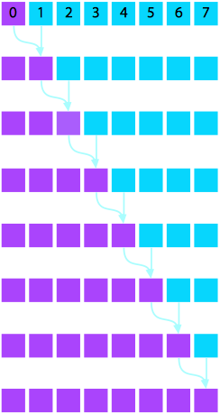 |
Parallel Version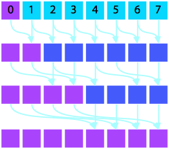 |
Basic Process
- Determine algorithms
- Decide on decomposition of computation into work and data units
- Decide on assignment of these units to processors
- Express decisions in language available for the machine
Tips
Architect a new parallel top-level structure rather than parallelizing a sequential program
Insert existing sequential code where appropriate
Refactor a portion of the sequential code into a parallel structure
Rewrite the remainder
Express algorithms in terms of $N$ and $P$.
Visualize data flow, not control flow, to reveal dependencies.
Exercise
- Implement the parallel prefix sum algorithm depicted graphically above. Feel free to copy code snippets from earlier to structure your code and then make it work.
%%file parprefix.c
// your code here
Writing Scientific Code
What else is (or should be) standard?
(Suggestions aggregated from Jay Alameda, Mark van Moers, and Neal Davis.)
Take the time to learn your development environment of choice well—there are language-aware code editors including code completion: IDEs (Eclipse, XCode),
vi(YouCompleteMe),emacs.Write self-documenting code: good variable and function names that follow a convention.
Modularize your code as much as practical.
Always include certain standard files when distributing your software:
README,INSTALL,CITATION,LICENSE.Use a compilation system: GNU Autotools (
./configure; make; make install), CMake, etc. (This also lets you query the hardware to optimize at compile time.)Use version control: Git, SVN, Mercurial, etc.
Use an issue-tracking system: GitHub issues, Bugzilla, etc.
Develop and use a unit-testing scheme (even a simple one).
Don't reinvent the wheel—find existing libraries: Boost, SciPy, Netlib, Scalapack, PETSc, etc.
Use configuration files and command-line flags rather than hard-coding values.
Compile with all debug flags set (
-Wall -Werror -g), and aim to compile with zero warnings.Don't create new file formats: find something existing that works (
HDF5,PDB,XYZ, etc.).Have a long-term data management plan (now a requirement for NSF, other grants).
Carry out studies of the strong and weak scaling, as well as profiling so that you aren't wasting cluster cycles.
Debugging Scientific Code

Now we come to one of the horrible truths about life and scientific computing: working code isn't necessarily correct code. Debugging is a much larger subject than we will be able to satisfactorily cover today, but I would like to give a ten-thousand-foot view of the subject as it applies to scientific computing.
There are a few general maxims I've picked up from various sources over the years:
Nobody gets it right the first time, [including you]. (Lynne Williams)
Premature optimization is the root of all evil. (Donald Knuth)
Confusion is a clue that something is wrong—don't ignore it. (Eliezer Yudkowsky paraphrase)
Checkpoint often.
First, learn to use debugging and profiling tools. Two that are supported on Campus Cluster are gdb and valgrind. gdb, the GNU Debugger, is designed to work with many programming languages besides C, but it can be painful to get it to work with a parallel program. Actually, any parallel debugging is painful.
The other tool, valgrind, monitors memory behavior. It can detect cache misses, memory leaks, and other problems which can lead to poor code performance and excessive memory demand.
Resources
DeinoMPI documentation. The most complete and thorough documentation (with examples) of MPI-2 functions.
//  THIS CODE OUTPUTS THE RESULTS SERIALLY TO DISK FROM EACH PROCESS.
    //  Write the final condition out to disk and terminate.
    //  Parallel I/O, while supported by MPI, is a whole other ball game and we won't go into here.
    //  Thus we will gather all of the data to process rank 0 and output it from there.
    double phi_all[size*base][size*base];
    //MPI_Send(&phi[0][0], base*N*base*N, MPI_DOUBLE

    FILE* f;
    char filename[16];
    sprintf(filename, "./data-%d.txt", rank_id);
    f = fopen(filename, "w"); // wb -write binary
    if (f != NULL) {
        for (int i = 0; i < size; i++) {
            for (int j = 0; j < size; j++) {
                fprintf(f, "%f\t", phi[i][j]);
            }
            fprintf(f, "\n");
        }
        fclose(f);
    } else {
        //failed to create the file
    }
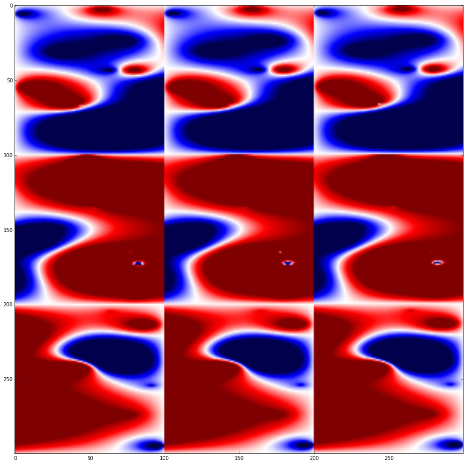
# Use Python to visualize the result quickly.
import numpy as np
import matplotlib as mpl
import matplotlib.pyplot as plt
from matplotlib import cm
%matplotlib inline
#mpl.rcParams['figure.figsize']=[20,20]

N = 9
data = []
grdt = []
for i in range(0, N):
    data.append(np.loadtxt('./data-%d.txt'%i))
    grdt.append(np.gradient(data[-1]))

fig, axes = plt.subplots(nrows=(int)(np.sqrt(N)), ncols=(int)(np.sqrt(N)), figsize=(12,12))
for i in range(0, (int)(np.sqrt(N))):
    for j in range(0, (int)(np.sqrt(N))):
        axes[i][j].imshow(data[i*(int)(np.sqrt(N))+j].T, cmap=cm.seismic, vmin=-3.5e6, vmax=3.5e6, extent=[-1,1,-1,1])
        #axes[i][j].contour(data[i*(int)(np.sqrt(N))+j].T, cmap=cm.bwr, vmin=-1.5e6, vmax=1.5e6, levels=np.arange(-1e7,1e7+1,2e5))
fig.show()
This code doesn't correctly handle the merge of data, instead spreading it out across segments twice as long and half as tall as the array.
//  Write the final condition out to disk and terminate.
//  Parallel I/O, while supported by MPI, is a whole other ball game and we won't go into here.
//  Thus we will gather all of the data to process rank 0 and output it from there.
double phi_all[size*base][size*base];
//MPI_Gather(&phi[0][0], size*size, MPI_DOUBLE, &phi_all[0][0], size*size, MPI_DOUBLE, 0, MPI_COMM_WORLD);
//  This version of the code ^ incorrectly orders the processor output.  We actually have to transpose each process's
//  data into a column-major format to get everything aligned properly.
double phi_new[size][size];
for (int i = 0; i < size; i++) {
    for (int j = 0; j < size; j++) {
        phi_new[j][i] = phi[i][j];
    }
}
if (rank_id==0) { printf("%d\n", rank_id);
for (int i = 0; i < size; i++) {
    for (int j = 0; j < size; j++) {
        printf("%f\t", phi[i][j]);
    }
    printf("\n");
}}MPI_Barrier(MPI_COMM_WORLD);
if (rank_id==1) { printf("%d\n", rank_id);
for (int i = 0; i < size; i++) {
    for (int j = 0; j < size; j++) {
        printf("%f\t", phi[i][j]);
    }
    printf("\n");
}}MPI_Barrier(MPI_COMM_WORLD);
if (rank_id==2) { printf("%d\n", rank_id);
for (int i = 0; i < size; i++) {
    for (int j = 0; j < size; j++) {
        printf("%f\t", phi[i][j]);
    }
    printf("\n");
}}MPI_Barrier(MPI_COMM_WORLD);
if (rank_id==3) { printf("%d\n", rank_id);
for (int i = 0; i < size; i++) {
    for (int j = 0; j < size; j++) {
        printf("%f\t", phi[i][j]);
    }
    printf("\n");
}}MPI_Barrier(MPI_COMM_WORLD);
MPI_Gather(&phi[0][0], size*size, MPI_DOUBLE, &phi_all[0][0], size*size, MPI_DOUBLE, 0, MPI_COMM_WORLD);
printf("\n\n\n");
if (rank_id == 0) {
    FILE* f;
    char filename[16];
    f = fopen("data.txt", "w"); // wb -write binary
    if (f != NULL) {
        for (int i = 0; i < base*size; i++) {
            for (int j = 0; j < base*size; j++) {
                fprintf(f, "%f\t", phi_all[i][j]);
                printf("%f\t", phi_all[i][j]);
            }
            fprintf(f, "\n");
            printf("\n");
        }
        fclose(f);
    } else {
        //failed to create the file
    }
}

List of MPI Functions
Initialization & Cleanup
MPI_Init
MPI_Finalize
MPI_Abort
MPI_Comm_rank
MPI_Comm_size
MPI_COMM_WORLD
MPI_Wtime
Message Passing
MPI_Status
MPI_Probe
Point-to-Point
We didn't discuss the mysterious "other" ways of sending messages mentioned earlier. These are they—other modes include explicit buffering (B), ready sending (so a matching receive must have already posted) (R), and synchronous sending (best for efficiency) (S). (ref)
MPI_Send
MPI_Bsend
MPI_Ssend
MPI_Rsend
MPI_Isend
MPI_Ibsend
MPI_Irsend
MPI_Recv
MPI_Irecv
MPI_Sendrecv
Collective
MPI_Bcast
MPI_Gather
MPI_Scatter
MPI_Allgather x{v}
MPI_Allreduce
MPI_Alltoall x{w,v}
xMPI_Reduce_scatter
xMPI_Scan
MPI_Barrier
Advanced
Derived Datatypes and Operations
MPI_Pack
MPI_Type_vector
MPI_Type_contiguous
MPI_Type_commit
MPI_Type_free
MPI_Op_create
MPI_User_function
MPI_Op_free
Robey’s Kahan sum, http://www.sciencedirect.com/science/article/pii/S0167819111000238
MPI_Comm_create
MPI_Scan
MPI_Exscan
MPI_Comm_free
I/O
MPI_File_*
One-Sided Communication MPI_Put write to remote memory MPI_Get read from remote memory MPI_Accumulate reduction op on same memory across multiple tasks