Probabilistic Programming in Python
Thomas Wiecki
@twiecki
Quantopian Inc.
In [65]:
from IPython.display import YouTubeVideo
YouTubeVideo("WESld11iNcQ")
Out[65]:
In [19]:
from IPython.display import Image
import prettyplotlib as ppl
from prettyplotlib import plt
import numpy as np
import scipy as sp
import seaborn as sns
sns.set_context('talk')
from matplotlib import rc
rc('font',**{'family':'sans-serif','sans-serif':['Helvetica'], 'size': 22})
rc('xtick', labelsize=12)
rc('ytick', labelsize=12)
## for Palatino and other serif fonts use:
#rc('font',**{'family':'serif','serif':['Palatino']})
rc('text', usetex=True)
%matplotlib inline

from IPython.html import widgets # Widget definitions
from IPython.display import display # Used to display widgets in the notebook
from IPython.html.widgets import interact, interactive
from IPython.display import clear_output, display, HTML

def gen_plot(success=(0, 100), failure=(0, 100)):
    alpha = 5 + success
    beta = 5 + failure
    fig = plt.figure(figsize=(8, 6))
    x = np.linspace(0, 1, 100)
    ax = fig.add_subplot(111, xlabel='Chance of success (beating the market)',
                         ylabel='Probability of hypothesis',
                         title=r'Posterior probability distribution of $\theta$')
    ax.plot(x, sp.stats.beta(alpha, beta).pdf(x), linewidth=3.)
    ax.set_xticklabels(['0\%', '20\%', '40\%', '60\%', '80\%', '100\%']);
In [5]:
from IPython.display import Image
import prettyplotlib as ppl
from prettyplotlib import plt
import numpy as np
import scipy as sp
import seaborn as sns
sns.set_context('talk')
from matplotlib import rc
rc('font',**{'family':'sans-serif','sans-serif':['Helvetica'], 'size': 22})
rc('xtick', labelsize=12)
rc('ytick', labelsize=12)
## for Palatino and other serif fonts use:
#rc('font',**{'family':'serif','serif':['Palatino']})
rc('text', usetex=True)
%matplotlib inline

from IPython.html import widgets # Widget definitions
from IPython.display import display # Used to display widgets in the notebook
from IPython.html.widgets import interact, interactive
from IPython.display import clear_output, display, HTML
About me
- PhD candidate at Brown studying decision making using Bayesian modeling.
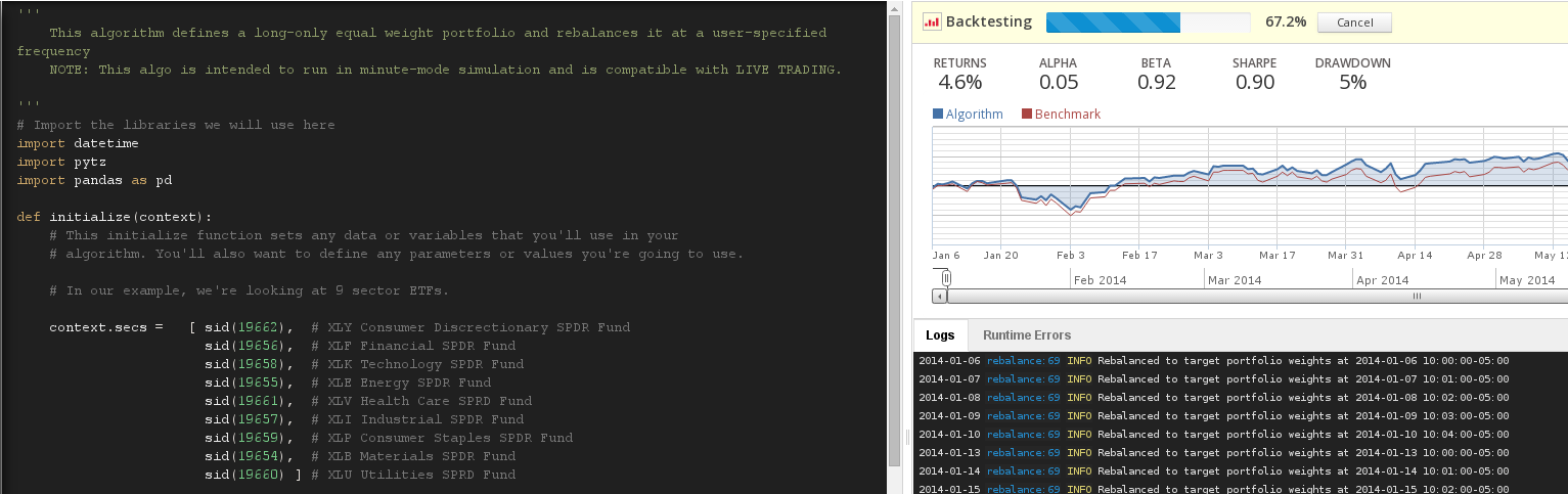
- Quantitative Researcher at Quantopian Inc: Building the world's first algorithmic trading platform in the web browser.
Why should you care about Probabilistic Programming?
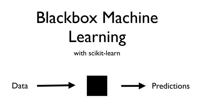 Source: Olivier Grisel's talk on ML
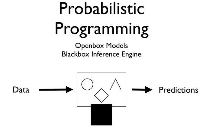 Source: Olivier Grisel's talk on ML
Data might look like this
In [38]:
from IPython.display import Image
import prettyplotlib as ppl
from prettyplotlib import plt
import numpy as np
import scipy as sp
import seaborn as sns
sns.set_context('talk')
from matplotlib import rc
rc('font',**{'family':'sans-serif','sans-serif':['Helvetica'], 'size': 22})
rc('xtick', labelsize=12)
rc('ytick', labelsize=12)
## for Palatino and other serif fonts use:
#rc('font',**{'family':'serif','serif':['Palatino']})
rc('text', usetex=True)
%matplotlib inline

from IPython.html import widgets # Widget definitions
from IPython.display import display # Used to display widgets in the notebook
from IPython.html.widgets import interact, interactive
from IPython.display import clear_output, display, HTML
In [62]:
np.random.seed(9)
algo_a = sp.stats.bernoulli(.5).rvs(10) # 10 samples from 50% chance of beating the market
algo_b = sp.stats.bernoulli(.6).rvs(10) # 10 samples from 60% chance of beating the market

print 'Beat the market algo A: ', algo_a
print 'Beat the market algo B: ', algo_b
Beat the market algo A:  [0 1 0 0 0 0 0 0 0 0]
Beat the market algo B:  [1 0 0 1 0 1 0 0 1 0]
The simplest answer
- Take the mean.
- This is equivalent to the maximum likelihood estimate, so statistically not a bad idea.
In [212]:
print 'Probability algo A beating the market = %.0f%%'
% (np.mean(algo_a) * 100)
print 'Probability algo B beating the market = %.0f%%'
% (np.mean(algo_b) * 100)
Probability algo A beating the market = 10%
Probability algo B beating the market = 40%
In [63]:
def run_exp():
    # Generate 50 random binary variables with probability = 0.5
    test_a = sp.stats.bernoulli(.5).rvs(50)
    test_b = sp.stats.bernoulli(.5).rvs(50)

    for i in range(2, 50):
        # Run statistical t-test
        _, p = sp.stats.ttest_ind(test_a[:i], test_b[:i])
        if p < 0.05:
            return True

    return False

p_sign_result = np.mean([run_exp() for i in range(1000)])

print 'Probability of getting significant result even though no\n difference exists = %.2f%%' % (p_sign_result * 100)
Probability of getting significant result even though no
 difference exists = 36.60%
What is Bayesian statistics?
- At the core: formula to update our beliefs after having observed data (Bayes formula)
- Implies that we have a prior belief about the world.
- Updated beliefs after observing data is called posterior.
- Beliefs are represented using random variables.

Let's define a prior for our random variable $\theta$
In [183]:
def gen_plot(successes=(0, 100, 1), failures=(0, 100, 1)):
    alpha_prior=5
    beta_prior=5
    if successes == 0 and failures == 0:
        title = r'Prior probability distribution on $\theta$'
    else:
        title = r'Posterior probability distribution of $\theta$ after having seen data'

    alpha = alpha_prior + successes
    beta = beta_prior + failures
    x = np.linspace(0, 1, 201)
    fig = plt.figure(figsize=(8, 6))
    ax = fig.add_subplot(111, xlabel=r'Chance of success (profit or conversion)',
                         ylabel=r'Probability',
                         title=title)
    ax.plot(x, sp.stats.beta(alpha, beta).pdf(x), linewidth=3.)
    ax.set_xticklabels([r'0\%', r'20\%', r'40\%', r'60\%', r'80\%', r'100\%']);

    return
In [15]:
def gen_plot(success=(0, 100), failure=(0, 100)):
    alpha = 5 + success
    beta = 5 + success
    fig = plt.figure(figsize=(8, 6))
    x = np.linspace(0, 1, 100)
    ax = fig.add_subplot(111, xlabel='Chance of success (beating the market)',
                         ylabel='Probability of hypothesis',
                         title=r'Posterior probability distribution of $\theta$')
    ax.plot(x, sp.stats.beta(alpha, beta).pdf(x), linewidth=3.)
    ax.set_xticklabels(['0\%', '20\%', '40\%', '60\%', '80\%', '100\%']);
In [16]:
gen_plot(0, 0)

In [64]:
interactive(gen_plot)

Where's the catch?
In most interesting cases, we can't solve what is inside the Bayesian box.
Probabilistic Programming
- If we can't solve something, approximate it.
- Markov-Chain Monte Carlo (MCMC) instead draws samples from the posterior.
- Fortunately, this algorithm can be applied to almost any model.
In [143]:
def plot_approx():
    from scipy import stats
    fig = ppl.plt.figure(figsize=(14, 6))
    x_plot = np.linspace(0, 1, 200)
    ax1 = fig.add_subplot(121, title='What we want', ylim=(0, 2.5))# , xlabel=r'$\theta$', ylabel=r'$P(\theta)$')
    ppl.plot(ax1, x_plot, stats.beta(4, 4).pdf(x_plot), linewidth=4.)
    ax2 = fig.add_subplot(122, title='What we get', xlim=(0, 1), ylim=(0, 2300))#, xlabel=r'\theta', ylabel='\# of samples')
    ax2.hist(stats.beta(4, 4).rvs(20000), bins=20);
Approximating the posterior with MCMC sampling
In [144]:
plot_approx()

PyMC3
- Probabilistic Programming framework written in Python.
- Allows for construction of probabilistic models using intuitive syntax.
- Features advanced MCMC samplers.
- Just-in-time compiled by Theano.
- Extensible: easily incorporates custom MCMC algorithms and unusual probability distributions.
- Written by: John Salvatier, Chris Fonnesbeck, Thomas Wiecki
- Currently still in alpha (few bugs but mainly missing docs).
Some necessary formalism:
$\theta_a \sim Beta(5, 5)$
$\theta_b \sim Beta(5, 5)$
$data_a \sim Bernoulli(\theta_a)$
$data_b \sim Bernoulli(\theta_b)$
- $\theta$ represents the unkown cause we want to infer, but can't observe directly.
- We write a generative story of how this unknown cause relates to observable data.
- Use Bayes to invert this generative story and infer hidden causes from observations -- updating our beliefs about $\theta$.
In [206]:
np.random.seed(9)
algo_a = sp.stats.bernoulli(.5).rvs(300) # 50% profitable days
algo_b = sp.stats.bernoulli(.6).rvs(300) # 60% profitable days
Chance of beating the market algo A:  0.493333333333
Chance of beating the market algo B:  0.6
In [207]:
import pymc as pm
model = pm.Model()
with model: # model specifications in PyMC3 are wrapped in a with-statement
    # Define random variables
    theta_a = pm.Beta('theta_a', alpha=5, beta=5) # prior
    theta_b = pm.Beta('theta_b', alpha=5, beta=5) # prior

    # Define how data relates to unknown causes
    data_a = pm.Bernoulli('observed A',
                          p=theta_a,
                          observed=algo_a)

    data_b = pm.Bernoulli('observed B',
                          p=theta_b,
                          observed=algo_b)

    # Inference!
    start = pm.find_MAP() # Find good starting point
    step = pm.Slice() # Instantiate MCMC sampling algorithm
    trace = pm.sample(10000, step, start=start, progressbar=False) # draw posterior samples using slice sampling
In [209]:
sns.distplot(trace['theta_a'], label=r'$\theta_a$')
sns.distplot(trace['theta_b'], label=r'$\theta_b$')
plt.title('Posteriors')
plt.legend()
Out[209]:
<matplotlib.legend.Legend at 0xf6ef250>

Hypothesis testing is trivial
In [208]:
p_b_better_than_a = np.mean(trace['theta_a'] < trace['theta_b'])
print 'Probability that algo B is better than A = %.2f%%' % (p_b_better_than_a * 100)
Probability that algo B is better than A = 99.11%
Advanced example -- hierarchical models
- Consider that instead of 2 algorithms, we have 20.
- Before we considered that $\theta_a$ and $\theta_b$ are completely independent.
- In reality, while they will probably be different, they will also have similarities.
- We can use hierarchical modeling to infer individual algorithms, but also their group distribution.
Unpooled

Pooled

Partially pooled -- hierarchical

In [247]:
np.random.seed(9)
algos = []
algos_idx = []
samples = 300
for i, p_algo in enumerate(sp.stats.beta(10, 10).rvs(20)):
    algos.append(sp.stats.bernoulli(p_algo).rvs(samples))
    algos_idx.append(np.ones(samples) * i)

algos = np.asarray(algos)
algos_idx = np.asarray(algos_idx, dtype=np.int)
print algos.shape
print algos
print algos_idx
(20, 300)
[[0 1 1 ..., 1 0 0]
 [0 1 1 ..., 0 1 0]
 [1 1 1 ..., 1 1 1]
 ...,
 [1 0 0 ..., 1 0 1]
 [0 1 1 ..., 0 0 0]
 [1 1 0 ..., 0 1 0]]
[[ 0  0  0 ...,  0  0  0]
 [ 1  1  1 ...,  1  1  1]
 [ 2  2  2 ...,  2  2  2]
 ...,
 [17 17 17 ..., 17 17 17]
 [18 18 18 ..., 18 18 18]
 [19 19 19 ..., 19 19 19]]
In [248]:
with pm.Model() as model: # model specifications in PyMC3 are wrapped in a with-statement
    # Define random variables
    grp_mean = pm.Beta('grp mean', alpha=2, beta=2) # prior
    grp_scale = pm.Gamma('grp scale', alpha=1, beta=10./10**2) # prior

    # Transform
    alpha = grp_mean * grp_scale
    beta = (1 - grp_mean) * grp_scale

    # Individual random variables, vector of lenght 20
    theta = pm.Beta('theta', alpha=alpha, beta=beta, shape=20)

    # Define how data relates to unknown causes
    data = pm.Bernoulli('observed',
                        p=theta[algos_idx],
                        observed=algos)

    # Inference!
    start = pm.find_MAP() # Find good starting point
    step = pm.NUTS (scaling=start) # Instantiate MCMC sampling algorithm
    trace = pm.sample(10000, step, start=start, progressbar=False)[:2000] # draw posterior samples using slice sampling
In [249]:
pm.traceplot(trace);

Conclusions
- Probabilistic Programming allows you to tell a genarative story.
- Blackbox inference algorithms allow estimation of complex models.
- PyMC3 puts advanced samplers at your fingertips.
Outstanding Issues
Scalability
- Variational Inference
- see also Max Welling's work for scaling MCMC
Usability
- still too difficult to use
- wanted: library on top of PyMC3 with common models
Further reading
- Quantopian -- Develop trading algorithms in Python in your browser.
- My blog on all things Bayesian
- Twitter: @twiecki
- Probilistic Programming for Hackers -- IPython Notebook book on Bayesian stats using PyMC2.
- Doing Bayesian Data Analysis -- Great book by Kruschke.
- Get PyMC3 alpha
- IPython Notebook underlying this talk