import theme
theme.load_style()
Introducing the IPython Notebook
This lecture is an adaptation of the lecture at Teaching Numerics with Notebooks and is covered by the following license
 Creative Commons Attribution 4.0 International License. All code examples are also licensed under the MIT license.
What is this?
This is a gentle introduction to the IPython Notebook aimed at lecturers who wish to incorporate it in their teaching, written in an IPython Notebook. This presentation adapts material from the IPython official documentation.
What is an IPython Notebook?
An IPython Notebook is a:
[A] Interactive environment for writing and running code
[B] Weave of code, data, prose, equations, analysis, and visualization
[C] Tool for prototyping new code and analysis
[D] Reproducible workflow for scientific research
[E] All of the above
[E] All of the above
How Do I Open an IPython Notebook?
Open a command prompt and execute
ipython notebook
and an IPython Notebook server will start and launch a viewer in the default web browser. Notebooks found in the working directory will show up in the list of notebooks.
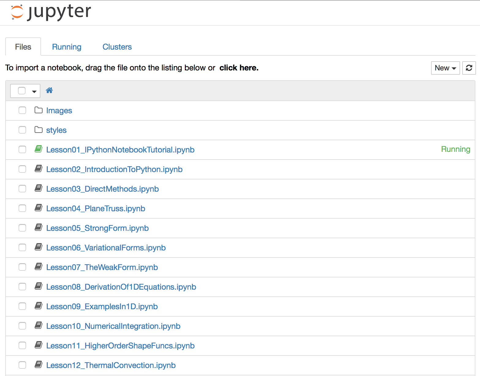
Example
For example, navigating to the course Lessons directory and executing ipython notebook will launch a browser window similar to that shown below
Writing and Running Code
The IPython Notebook consists of an ordered list of cells.
There are three important cell types:
- Code
- Markdown
- Raw NBConvert
Code Cells
# This is a code cell made up of Python comments
# We can execute it by clicking on it with the mouse
# then clicking the "Run Cell" button
# A comment is a pretty boring piece of code
# This code cell generates "Hello, World" when executed

print "Hello, World"
Hello, World
Code Cells
# Code cells can also generate graphical output
%matplotlib inline
import matplotlib
matplotlib.pyplot.hist([0, 1, 2, 2, 3, 3, 3, 4, 4, 4, 10]);

Modal editor
Starting with IPython 2.0, the IPython Notebook has a modal user interface. This means that the keyboard does different things depending on which mode the Notebook is in. There are two modes: edit mode and command mode.
Edit mode
Edit mode is indicated by a green cell border and a prompt showing in the editor area:

When a cell is in edit mode, you can type into the cell, like a normal text editor.
Command mode
Command mode is indicated by a grey cell border:

When you are in command mode, you are able to edit the notebook as a whole, but not type into individual cells. Most importantly, in command mode, the keyboard is mapped to a set of shortcuts that let you perform notebook and cell actions efficiently. For example, if you are in command mode and you press c, you will copy the current cell - no modifier is needed.
Mouse navigation
All navigation and actions in the Notebook are available using the mouse through the menubar and toolbar, which are both above the main Notebook area:

Cell Clicking
The first idea of mouse based navigation is that cells can be selected by clicking on them. The currently selected cell gets a grey or green border depending on whether the notebook is in edit or command mode. If you click inside a cell's editor area, you will enter edit mode. If you click on the prompt or output area of a cell you will enter command mode.
If you are running this notebook in a live session (not on http://nbviewer.ipython.org) try selecting different cells and going between edit and command mode. Try typing into a cell.
Current Selection
The second idea of mouse based navigation is that cell actions usually apply to the currently selected cell. Thus if you want to run the code in a cell, you would select it and click the "Play" button in the toolbar or the "Cell:Run" menu item. Similarly, to copy a cell you would select it and click the "Copy" button in the toolbar or the "Edit:Copy" menu item. With this simple pattern, you should be able to do most everything you need with the mouse.
Markdown Rendering
Markdown and heading cells have one other state that can be modified with the mouse. These cells can either be rendered or unrendered. When they are rendered, you will see a nice formatted representation of the cell's contents. When they are unrendered, you will see the raw text source of the cell. To render the selected cell with the mouse, click the "Play" button in the toolbar or the "Cell:Run" menu item. To unrender the selected cell, double click on the cell.
Keyboard Navigation
The modal user interface of the IPython Notebook has been optimized for efficient keyboard usage. This is made possible by having two different sets of keyboard shortcuts: one set that is active in edit mode and another in command mode.
The most important keyboard shortcuts are enter, which enters edit mode, and esc, which enters command mode.
In edit mode, most of the keyboard is dedicated to typing into the cell's editor. Thus, in edit mode there are relatively few shortcuts:
Keyboard Navigation
In command mode, the entire keyboard is available for shortcuts.
Here the rough order in which the IPython Developers recommend learning the command mode shortcuts:
- Basic navigation:
enter,shift-enter,up/k,down/j - Saving the notebook:
s - Cell types:
y,m,1-6,t - Cell creation and movement:
a,b,ctrl+k,ctrl+j - Cell editing:
x,c,v,d,z,shift+= - Kernel operations:
i,0
I suggest learning h first!
The IPython Notebook Architecture
So far, we have learned the basics of using IPython Notebooks.
For simple demonstrations, the typical user doesn't need to understand how the computations are being handled, but to successfully write and present computational notebooks, you will need to understand how the notebook architecture works.
A live notebook is composed of an interactive web page (the front end), a running IPython session (the kernel or back end), and a web server responsible for handling communication between the two (the, err..., middle-end)
A static notebook, as for example seen on NBViewer, is a static view of the notebook's content. The default format is HTML, but a notebook can also be output in PDF or other formats.
The centerpiece of an IPython Notebook is the "kernel", the IPython instance responsible for executing all code. Your IPython kernel maintains its state between executed cells.
x = 0
print x
0
x += 1
print x
1
Interacting with the Kernel
There are two important actions for interacting with the kernel. The first is to interrupt it. This is the same as sending a Control-C from the command line. The second is to restart it. This completely terminates the kernel and starts it anew. None of the kernel state is saved across a restart.
Markdown cells
Text can be added to IPython Notebooks using Markdown cells. Markdown is a popular markup language that is a superset of HTML. Its specification can be found here:
Markdown basics
Text formatting
You can make text italic or bold.
Itemized Lists
- One
- Sublist
- This
- Sublist - That - The other thing
- Sublist
- Two
- Sublist
- Three
- Sublist
Enumerated Lists
- Here we go
- Sublist
- Sublist
- There we go
- Now this
Blockquotes
To me programming is more than an important practical art. It is also a gigantic undertaking in the foundations of knowledge. -- Rear Admiral Grace Hopper
Links
Code
def f(x):
    """a docstring"""
    return x**2
You can also use triple-backticks to denote code blocks. This also allows you to choose the appropriate syntax highlighter.
if (i=0; i<n; i++) {
  printf("hello %d\n", i);
  x += 4;
}
Tables
| Time (s) | Audience Interest |
|---|---|
| 0 | High |
| 1 | Medium |
| 5 |
Images

YouTube
from IPython.display import YouTubeVideo YouTubeVideo('vW_DRAJ0dtc')
Other HTML
Be Bold!
Mathematical Equations
Courtesy of MathJax, you can beautifully render mathematical expressions, both inline: $e^{i\pi} + 1 = 0$, and displayed:
$$e^x=\sum_{i=0}^\infty \frac{1}{i!}x^i$$Equation Environments
You can also use a number of equation environments, such as align:
A full list of available TeX and LaTeX commands is maintained by Dr. Carol Burns.
Other Useful MathJax Notes
- inline math is demarcated by
$ $, or\( \) - displayed math is demarcated by
$$ $$or\[ \] - displayed math environments can also be directly demarcated by
\beginand\end \newcommandand\defare supported, within areas MathJax processes (such as in a\[ \]block)- equation numbering is not officially supported, but it can be indirectly enabled
A Note about Notebook Security
By default, a notebook downloaded to a new computer is untrusted
- HTML and Javascript in Markdown cells is now never executed
- HTML and Javascript code outputs must be explicitly re-executed
- Some of these restrictions can be mitigrated through shared accounts (Sage MathCloud) and secrets
More information on notebook security is in the IPython Notebook documentation
Magics
IPython kernels execute a superset of the Python language. The extension functions, commonly referred to as magics, come in two variants.
Line Magics
- A line magic looks like a command line call. The most important of these is
%matplotlib inline, which embeds all matplotlib plot output as images in the notebook itself.
%matplotlib inline
%whos
Variable     Type      Data/Info
--------------------------------
matplotlib   module    <module 'matplotlib' from<...>matplotlib/__init__.pyc'>
x            int       1
Cell Magics
- A cell magic takes its entire cell as an argument. Although there are a number of useful cell magics, you may find
%%timeitto be useful for exploring code performance.
%%timeit

import numpy as np
np.sum(np.random.rand(1000))
The slowest run took 464.75 times longer than the fastest. This could mean that an intermediate result is being cached
100000 loops, best of 3: 17.6 µs per loop
Interacting with the Command Line
IPython supports one final trick, the ability to interact directly with your shell by using the ! operator.
!ls
Images                                       Lesson11_HigherOrderShapeFuncs.ipynb
Lesson01_IPythonNotebookTutorial.ipynb       Lesson12_ThermalConvection.ipynb
Lesson01_IPythonNotebookTutorial.slides.html Lesson13_AdvectionDiffusion.ipynb
Lesson02_IntroductionToPython.ipynb          Lesson14_NonlinearMaterials.ipynb
Lesson03_DirectMethods.ipynb                 Lesson15_ErrorAnalysis.ipynb
Lesson04_PlaneTruss.ipynb                    Lesson16_MethodOfManufacturedSolutions.ipynb
Lesson05_StrongForm.ipynb                    Lesson17_EulerBernouliBeamElement.ipynb
Lesson06_VariationalForms.ipynb              Lesson20_GeneralizedBoundaryConditions.ipynb
Lesson07_TheWeakForm.ipynb                   MathematicalPreliminaries.ipynb
Lesson08_DerivationOf1DEquations.ipynb       styles
Lesson09_ExamplesIn1D.ipynb                  theme.py
Lesson10_NumericalIntegration.ipynb          theme.pyc
x = !ls
print x
['Images', 'Lesson01_IPythonNotebookTutorial.ipynb', 'Lesson01_IPythonNotebookTutorial.slides.html', 'Lesson02_IntroductionToPython.ipynb', 'Lesson03_DirectMethods.ipynb', 'Lesson04_PlaneTruss.ipynb', 'Lesson05_StrongForm.ipynb', 'Lesson06_VariationalForms.ipynb', 'Lesson07_TheWeakForm.ipynb', 'Lesson08_DerivationOf1DEquations.ipynb', 'Lesson09_ExamplesIn1D.ipynb', 'Lesson10_NumericalIntegration.ipynb', 'Lesson11_HigherOrderShapeFuncs.ipynb', 'Lesson12_ThermalConvection.ipynb', 'Lesson13_AdvectionDiffusion.ipynb', 'Lesson14_NonlinearMaterials.ipynb', 'Lesson15_ErrorAnalysis.ipynb', 'Lesson16_MethodOfManufacturedSolutions.ipynb', 'Lesson17_EulerBernouliBeamElement.ipynb', 'Lesson20_GeneralizedBoundaryConditions.ipynb', 'MathematicalPreliminaries.ipynb', 'styles', 'theme.py', 'theme.pyc']
A Note about Notebook Version Control
The IPython Notebook is stored using canonicalized JSON for ease of use with version control systems.
There are two things to be aware of:
By default, IPython embeds all content and saves kernel execution numbers. You may want to get in the habit of clearing all cells before committing.
As of IPython 2.0, all notebooks are signed on save. This increases the chances of a commit collision during merge, forcing a manual resolution. Either signature can be safely deleted in this situation.