In [6]:
import syde556
a = syde556.Ensemble(neurons=50, dimensions=1)

x = numpy.linspace(-1, 1, 100)
ideal = x
d = a.compute_decoder(x, ideal, noise=0.2)
A, xhat = a.simulate_rate(x, d)
print 'RMSE:', sqrt(mean((ideal-xhat)**2))
subplot(2,1,1)
plot(x, ideal, color='k')
plot(x, xhat, color='b')
subplot(2,1,2)
plot(x, A)
show()
RMSE: 0.0141812072763

- What about $f(x)=10x$? or larger numbers?
$f(x)=x^2$
In [19]:
import syde556
a = syde556.Ensemble(neurons=50, dimensions=1)

x = numpy.linspace(-1, 1, 100)
ideal = x**2
d = a.compute_decoder(x, ideal, noise=0.2)
A, xhat = a.simulate_rate(x, d)
print 'RMSE:', sqrt(mean((ideal-xhat)**2))
subplot(2,1,1)
plot(x, ideal, color='k')
plot(x, xhat, color='b')
subplot(2,1,2)
plot(x, A)
show()
RMSE: 0.0408841434153

Other exponents?
- $f(x)=x^3$
- $f(x)=x^4$
- $f(x)=x^5$
- $f(x)=x^0$
Polynomials?
- If it's fairly good at $f(x)=2x$ and fairly good at $f(x)=x^2$, what happens with $f(x)=x^2+2x$?
Other functions?
$f(x)=e^{- (x-b)^2/(2c^2)}$
In [39]:
import syde556
a = syde556.Ensemble(neurons=100, dimensions=1)

x = numpy.linspace(-1, 1, 100)

c = 0.5
b = 0
ideal = exp(-(x-b)**2/(2*c**2))
d = a.compute_decoder(x, ideal, noise=0.2)
A, xhat = a.simulate_rate(x, d)
print 'RMSE:', sqrt(mean((ideal-xhat)**2))
subplot(2,1,1)
plot(x, ideal, color='k')
plot(x, xhat, color='b')
subplot(2,1,2)
plot(x, A)
show()
RMSE: 0.0292945716158

- What about different values of $c$?
The Decoder Calculation
- What are decoders good at?
- How do we compute decoders?
- Here's the simple noise-free case:
- $\Gamma=A^T A$ and $\Upsilon=A^T f(x)$
- $ d = \Gamma^{-1} \Upsilon $
- Consider the $\Gamma$ matrix
- This is known as a Gram matrix
- Measure of similarity of neural responses (correlation matrix)
- Tells us about the representation of the vector space by the neurons
- Stepping through the decoder calculation:
- ideally, $X = A d$
- $A^T X = A^T A d$
- $(A^T A)^{-1} A^T X = d$
- In this ideal case, how do we take the inverse correctly?
- This is likely to be a singular matrix (lots of neurons have similar tuning curves)
- Less of an issue normally, since we take noise into account and add onto the diagonal
- Instead, let's do SVD to decompose and approximately invert the matrix
- Singular Value Decomposition
- In general, $B_{M,N}=U_{M,M} S_{M,N} V^T_{N,N}$ where $S$ is a diagonal matrix of singular values
- But here, $\Gamma$ is square and symmetric, so $\Gamma=U S U^T$ and the inverse of $\Gamma$ can be written as $U S^{-1} U^T$
- When $\Gamma$ in singular (or nearly so), then some elements of the diagonal of $S$ are zero (or very small), so the inverse has values that are infinite (or very large)
- The "Pseudo-inverse" is to say if $S_i=0$, then $S^{-1}_i=0$
Usefulness of SVD
- Regardless of the function we want to decode, we always invert the same $\Gamma$ matrix
- identity decoder is just the special case $f(x)=x$
- Understanding properties of $\Gamma$ can provide insight into all possible decodings from the populations's activity $A$
- The singular values $S$ tell us the importance of a particular $U$ vector, including
- the error if that $U$ vector was left out of the mapping
- relative to the variance of the population firing
- the amount of independent information about the population firing that could be extracted if we were only looking at the data projected onto that $U$ vector.
- In general, we can think of the magnitude of the singular value as telling us how relevant that $U$ vector is to the identity of the matrix we have decomposed
- Since the matrix we have decomposed is like the correlation matrix of the neuron tuning curves, the large singular values are the most important for accounting for the structure of those correlations
- The vectors in $U$ are orthogonal
- they are an ordered, orthogonal basis
- The original $\Gamma$ matrix was generated by a non-ordered, non-orthogonal basis: the neuron tuning curves
- Consider the neural activity for a particular $x$ value
- A row of the $A$ matrix
- The "activity space" of the neurons
- Because the neural responses are non-independently driven by some variable $x$, only a small part of the subspace of possible neural activity values is ever reached by the population
- the $\Gamma$ matrix, because it tells us the correlations between all neurons in the population, provides the information needed to determine that subspace
- That subspace is $U$
- So what?
- So, let's rotate our neural activity curves $A$ into this subspace and see what they look like.
- $\chi = A U$
- These will be the orthogonal functions we can decode, ordered by accuracy
In [95]:
import syde556
a = syde556.Ensemble(neurons=300, dimensions=1, seed=0)

x = numpy.linspace(-1, 1, 100)
ideal = x
d = a.compute_decoder(x, ideal, noise=0.2)
A, xhat = a.simulate_rate(x, d)

Gamma = numpy.dot(A.T, A)
U,S,V = numpy.linalg.svd(Gamma)

chi = numpy.dot(A, U)

for i in range(5):
    plot(x, chi[:,i], label='$\chi_%d$=%1.3g'%(i, S[i]), linewidth=3)
legend(loc='best', bbox_to_anchor=(1,1))
show()

- Does anybody recognize those functions?
In [97]:
subplot(1,2,1)
for i in range(5):
    plot(x, chi[:,i], linewidth=3)

subplot(1,2,2)
for i in range(5):
    plot(x, numpy.polynomial.legendre.legval(x, numpy.eye(5)[i]))
show()

- The Legendre polynomials
- Or at least scaled version thereof
- So we should be able to approximate any function that can be approximated by polynomials
- But remember that they are ordered by their singular values
- See how quickly the singular values drop off:
In [92]:
plot(S)
show()

- If you need higher and higher polynomials, you need many more neurons
Modifying that basis
- Are we stuck with this?
- What can we do to modify these bases functions?
In [40]:
import syde556
a = syde556.Ensemble(neurons=100, dimensions=1, seed=0,
                     intercept=(-0.3, 0.3))

x = numpy.linspace(-1, 1, 100)
ideal = x
d = a.compute_decoder(x, ideal, noise=0.2)
A, xhat = a.simulate_rate(x, d)

Gamma = numpy.dot(A.T, A)
U,S,V = numpy.linalg.svd(Gamma)

chi = numpy.dot(A, U)

figure()
plot(x, A)

figure()
for i in range(6):
    plot(x, chi[:,i], label='$\chi_%d$=%1.3g'%(i, S[i]), linewidth=3)
legend(loc='best', bbox_to_anchor=(1,1))
show()


- What about other distributions of intercepts?
- Changing these distributions also affects how much it gets better with more neurons
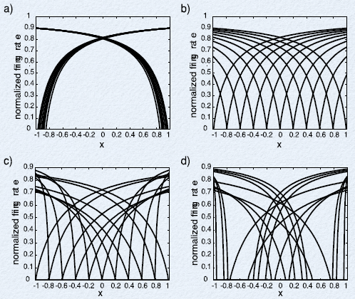

- Note that the accuracy curves are for $f(x)=x$
Higher dimensions
- Does this apply to vectors as well as scalars?
- Of course
- Same math, even
- Just a little harder to plot
In [36]:
import syde556
a = syde556.Ensemble(neurons=300, dimensions=2, seed=0)

x0 = numpy.linspace(-1,1,50)
x1 = numpy.linspace(-1,1,50)

x0, x1 = numpy.array(meshgrid(x0,x1))
x = numpy.array([numpy.ravel(x0), numpy.ravel(x1)])

d = a.compute_decoder(x, x, noise=0.2)
A, xhat = a.simulate_rate(x, d)

Gamma = numpy.dot(A.T, A)
U,S,V = numpy.linalg.svd(Gamma)

chi = numpy.dot(A, U)

index = 0
basis = chi[:,index]
basis.shape = 50,50

from mpl_toolkits.mplot3d.axes3d import Axes3D
fig = pylab.figure()
ax = fig.add_subplot(1, 1, 1, projection='3d')
p = ax.plot_surface(x0, x1, basis, linewidth=0, cstride=1, rstride=1, cmap=pylab.cm.jet)
pylab.title('Basis #%d (sv=%1.4g)'%(index, S[index]))
show()

- Again, we get the polynomials
- In general, we get cross-terms in the computable functions
- For the 2D case:
- $f(x)=a_0 + a_1 x_0 + a_2 x_1 + a_3 x_0^2 + a_4 x_1^2 + a_5 x_0 x_1 + ...$
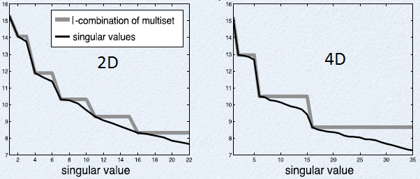
The grey line is constant for as many terms as should be at about the same accuracy level
In higher dimensions, higher order functions are even harder
This is all also going to be affected by distributions of encoders (as well as distributions of intercepts and maximum rates)
Given a function, can we automatically find good choices for tuning curves?
- In general, this is a difficult problem
- Indeed, we can cast this as exactly the standard multi-layer neural network learning problem
- But analyzing it this way gives us hints
General techniques
- If your function has a big zero area, see if you can get the tuning curves to also be zero in that area
- Smooth, broad functions are best
- For the special case of $f(x)=x_0 x_1$, arrange your encoders at $[1,1], [1,-1], [-1,-1], [-1, 1]$
In [ ]: