SYDE 556/750: Simulating Neurobiological Systems
Accompanying Readings: Chapter 6
Terry Stewart
Transformation
The story so far:
- The activity of groups of neurons can represnt variables $x$
- $x$ can be an aribitrary-dimension vector
- each neuron has a preferred vector $e$
- current going into each neuron is $J = \alpha e \cdot x + J^{bias}$
- we can interpret neural activity via $\hat{x}=\sum a_i d_i$
- for spiking neurons, we filter the spikes first: $\hat{x}=\sum (a_i(t)*h(t))d_i$
- to compute $d$, generate some $x$ values and find the optimal $d$ (assuming some amount of noise)
So far we've just talked about neural activity
What about connections between neurons?
Connecting neurons
- Up till now, we've always had the current going into a neuron be something we computed from $x$
- $J = \alpha e \cdot x + J^{bias}$
- This will continue to be how we handle inputs
- sensory neurons, for example
- or whatever's coming from the rest of the brain that we're not modelling (yet)
- But what about other groups of neurons?
- How do they end up getting exactly the amount of input current that we're assuming with $J = \alpha e \cdot x + J^{bias}$ ?
- Where does that current come from?
A communication channel
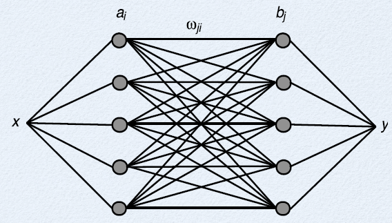
- Let's say we have two groups of neurons
- one group represents $x$
- one group represents $y$
- can we pass the value from one group of neurons to the other?
- Each neuron $i$ representing $x$ connects to each neuron $j$ representing $y$
- each connection has a weight $\omega_{ij}$
- total input to each neuron $j$ is the sum of the weighted outputs from the $i$ neurons
- $J_j = \sum_i a_i \omega_{ij} $
- We want the current $J_j$ to be the same current as we would have got from $J=\alpha e \cdot x + J^{bias}$
- can we find $\omega_{ij}$ values that would achieve this?
In [49]:
import numpy
import syde556
reload(syde556)


x, X = syde556.generate_signal(T=1, dt=0.001, rms=0.3, limit=10, seed=3)

N_i = 20
encoders_i = numpy.random.choice([1, -1], N_i)
intercepts_i = numpy.random.uniform(-0.95, 0.95, N_i)
max_rates_i = numpy.random.uniform(250, 300, N_i)
alpha_i, bias_i = syde556.find_alpha_and_bias(intercepts_i, max_rates_i)

N_j = 19
encoders_j = numpy.random.choice([1, -1], N_j)
intercepts_j = numpy.random.uniform(-0.95, 0.95, N_j)
max_rates_j = numpy.random.uniform(250, 300, N_j)
alpha_j, bias_j = syde556.find_alpha_and_bias(intercepts_j, max_rates_j)


A_i = syde556.activity(x, encoders_i, alpha_i, bias_i)
d_i = syde556.decoders(A_i, x, noise=0.1, dx=1.0/len(x))

A_j = syde556.activity(x, encoders_j, alpha_j, bias_j)
d_j = syde556.decoders(A_j, x, noise=0.1, dx=1.0/len(x))

xhat_i = numpy.dot(syde556.add_noise(A_i, 0.1), d_i)
xhat_j = numpy.dot(syde556.add_noise(A_j, 0.1), d_j)

t = numpy.arange(len(x))*0.001
figure(figsize=(8,4))
subplot(1,2,1)
plot(t, x, label='$x$')
plot(t, xhat_i, label='$\hat{x}$')
legend()
xlabel('time (seconds)')
ylabel('value')
ylim(-1.5, 1.0)
title('first population')

subplot(1,2,2)
plot(t, x, label='$y$')
plot(t, xhat_j, label='$\hat{y}$')
legend()
xlabel('time (seconds)')
ylabel('value')
ylim(-1.5, 1.0)
title('second population')

show()

- The computation we use for decoders is close to what we're looking for
- we want to feed in some amount of current $J_j$, but all we have are a bunch of activity values that we can added together
- so we find a weighted sum that closely approximates the desired $J_j$
In [50]:
weights = numpy.zeros((N_i, N_j))
for j in range(N_j):
    J_desired = alpha_j[j]*encoders_j[j]*x+bias_j[j]
    weights[:,j] = syde556.decoders(A_i, J_desired, noise=0.1, dx=1.0/len(x))

J_j = numpy.dot(A_i, weights)
A_j = syde556.lif(J_j)

xhat_j = numpy.dot(syde556.add_noise(A_j, 0.1), d_j)

figure(figsize=(8,4))
subplot(1,2,1)
plot(t, x, label='$x$')
plot(t, xhat_i, label='$\hat{x}$')
legend()
xlabel('time (seconds)')
ylabel('value')
ylim(-1.5, 1.0)
title('first population')

subplot(1,2,2)
plot(t, x, label='$y$')
plot(t, xhat_j, label='$\hat{y}$')
legend()
xlabel('time (seconds)')
ylabel('value')
ylim(-1.5, 1.0)
title('second population fed from first')

show()

- The basic trick is that we can use the algorithm to find decoders to find decoders that approximate value other than $x$
- We just replace $x$ with whatever we want
- $ \Upsilon_i = {1 \over 2} \int_{-1}^1 a_i x dx$
- $ \Gamma_{ij} = {1 \over 2} \int_{-1}^1 a_i a_j dx $
- $ d = \Gamma^{-1} \Upsilon $
- Notice that we don't even have to recompute $ \Gamma^{-1} $
- So consider finding the weights for the first neuron in the output population
- compute the desired current for each $x$ value: $J = \alpha e \cdot x + J^{bias}$
- find the decoders that give that $J$ value
- repeat for the other neurons
A shortcut
- Let's simplify the solving a bit
- First, get rid of $J^{bias}$
- Assume that the neurons are getting some constant background input at that level
- this value never changes, and it's randomly chosen anyway
- Now, the desired input current for each neuron $j$ is $J_j = \alpha_j e_j \cdot x$
- We want $J_j = \sum_i a_i \omega_{ij}$
- We already have the standard decoder that gives $\hat{x} = \sum_i a_i d_i$
- So what if we substitute in $\hat{x}$ for $x$?
- $J_j = \alpha_j e_j \cdot x$
- $J_j = \alpha_j e_j \cdot \sum_i a_i d_i$
- $J_j = \sum_i a_i (\alpha_j e_j \cdot d_i)$
- $\omega_{ij} = \alpha_j e_j \cdot d_i$
- In other words, we can get the entire weight matrix just by mupliplying the decoders from the first population with the encoders from the second population
- Instead of optimizing each set of connections individually
In [51]:
weights = numpy.outer(d_i, alpha_j*encoders_j)

J_j = numpy.dot(A_i, weights)+bias_j
A_j = syde556.lif(J_j)

xhat_j = numpy.dot(syde556.add_noise(A_j, 0.1), d_j)

figure(figsize=(8,4))
subplot(1,2,1)
plot(t, x, label='$x$')
plot(t, xhat_i, label='$\hat{x}$')
legend()
xlabel('time (seconds)')
ylabel('value')
ylim(-1.5, 1.0)
title('first population')

subplot(1,2,2)
plot(t, x, label='$y$')
plot(t, xhat_j, label='$\hat{y}$')
legend()
xlabel('time (seconds)')
ylabel('value')
ylim(-1.5, 1.0)
title('second population fed from first')

show()

- In fact, instead of computing $\omega_{ij}$ at all, it is (usually) more efficient to just do the multiplying
- saves a lot of memory space, since you don't have to store a giant weight matrix
In [52]:
J_j = numpy.outer(numpy.dot(A_i, d_i), alpha_j*encoders_j)+bias_j
- This means we get the exact same effect as having a weight matrix $\omega_{ij}$ if we just take the decoded value from one population and feed that into the next population using the normal encoding method
- these are numerically identical processes, since $\omega_{ij} = \alpha_j e_j \cdot d_i$
Spiking neurons
- The same approach works for spiking neurons
- Do exactly the same as before
- The $a_i(t)$ values are spikes, and we convolve with $h(t)$
Other transformations
- So this lets us take an $x$ value and feed it into another population
- passing information from one group of neurons to the next
- What about transforming that information in some way?
- instead of $y=x$, can we do $y=f(x)$?
- Let's try $y=2x$ to start
- We already have a decoder for $\hat{x}$, so how do we get a decoder for $\hat{2x}$?
- two ways
- either use $2x$ when computing $\Upsilon$
- or just multiply your standard decoder by $2$
In [3]:
import syde556

dt = 0.001
x = numpy.linspace(-1, 1, 1000)
A = syde556.Ensemble(neurons=25, dimensions=1)
B = syde556.Ensemble(neurons=23, dimensions=1)
decoder_A = A.compute_decoder(x, 2*x)
decoder_B = B.compute_decoder(x, x)

x, X = syde556.generate_signal(1.0, dt, rms=0.3, limit=5, seed=2)

spikes_A, x_A = A.simulate_spikes(x, decoder_A, tau=0.01)
spikes_B, x_B = B.simulate_spikes(x_A, decoder_B, tau=0.01)

figure()
t = numpy.arange(len(x))*dt
imshow(spikes_A.T, extent=(0,1.0,-1,1), aspect='auto', interpolation='none', cmap='binary')
plot(t, x_A)
plot(t, x)
title('population A')

figure()
imshow(spikes_B.T, extent=(0,1.0,-1,1), aspect='auto', interpolation='none', cmap='binary')
plot(t, x_B)
plot(t, 2*x)
title('population B')

show()


- What about a nonlinear function?
- $y = x^2$
In [160]:
import syde556

dt = 0.001
x = numpy.linspace(-1, 1, 1000)
A = syde556.Ensemble(neurons=25, dimensions=1)
B = syde556.Ensemble(neurons=23, dimensions=1)
decoder_A = A.compute_decoder(x, x**2)
decoder_B = B.compute_decoder(x, x)

x, X = syde556.generate_signal(1.0, dt, rms=0.3, limit=5, seed=2)

spikes_A, x_A = A.simulate_spikes(x, decoder_A, tau=0.01)
spikes_B, x_B = B.simulate_spikes(x_A, decoder_B, tau=0.01)

figure()
t = numpy.arange(len(x))*dt
imshow(spikes_A.T, extent=(0,1.0,-1,1), aspect='auto', interpolation='none', cmap='binary')
plot(t, x_A)
plot(t, x)
title('population A')

figure()
imshow(spikes_B.T, extent=(0,1.0,-1,1), aspect='auto', interpolation='none', cmap='binary')
plot(t, x_B)
plot(t, x**2)
title('population B')

show()


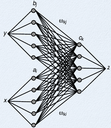
- We want the total current going into a $z$ neuron to be $J=\alpha e \cdot (x+y) + J^{bias}$
- How can we achieve this?
- Let's optimize again
- sample over $<x,y>$
- find $\omega$ for each connection that minimizes error
- Can we do this more efficiently?
- Again, substitute into the equation
- $J_k=\alpha_k e \cdot (x+y) + J_k^{bias}$
- $\hat{x} = \sum_i a_i d_i$
- $\hat{y} = \sum_j a_j d_j$
- $J_k=\alpha_k e_k \cdot (\sum_i a_i d_i+\sum_j a_j d_j) + J_k^{bias}$
- $J_k=\sum_i(\alpha_k e_k \cdot d_i a_i) + \sum_j(\alpha_k e_k \cdot d_j a_j) + J_k^{bias}$
- $J_k=\sum_i(\omega_{ik} a_i) + \sum_j(\omega_{jk} a_j) + J_k^{bias}$
- $\omega_{ik}=\alpha_k e_k \cdot d_i$ and $\omega_{jk}=\alpha_k e_k \cdot d_j$
- Putting multiple inputs into a neuron automatically gives us addition!
In [102]:
import syde556

dt = 0.001
x = numpy.linspace(-1, 1, 1000)
A = syde556.Ensemble(neurons=50, dimensions=1)
B = syde556.Ensemble(neurons=50, dimensions=1)
C = syde556.Ensemble(neurons=50, dimensions=1)

decoder_A = A.compute_decoder(x, x, noise=0.2)
decoder_B = B.compute_decoder(x, x, noise=0.2)
decoder_C = C.compute_decoder(x, x, noise=0.2)

x, X = syde556.generate_signal(1.0, dt, rms=0.2, limit=5, seed=2)
y, X = syde556.generate_signal(1.0, dt, rms=0.2, limit=5, seed=6)

spikes_A, xhat = A.simulate_spikes(x, decoder_A, tau=0.01)
spikes_B, yhat = B.simulate_spikes(y, decoder_B, tau=0.01)

spikes_C, zhat = C.simulate_spikes(xhat+yhat, decoder_C, tau=0.01)

figure()
t = numpy.arange(len(x))*dt
plot(t, x, label='$x$')
plot(t, y, label='$y$')
plot(t, x+y, label='$x+y$')
plot(t, zhat, label='$\hat{z}$')
legend(loc='best')

show()

Vectors
- Nothing changes
In [158]:
import syde556
reload(syde556)

dt = 0.001

A = syde556.Ensemble(neurons=50, dimensions=2)
B = syde556.Ensemble(neurons=50, dimensions=2)
C = syde556.Ensemble(neurons=50, dimensions=2)

x = numpy.random.normal(0, 0.5, size=(2,1000))
decoder_A = A.compute_decoder(x, x, noise=0.2)

decoder_B = B.compute_decoder(x, x, noise=0.2)
decoder_C = C.compute_decoder(x, x, noise=0.2)

x = numpy.zeros((2,1000))+numpy.array([0.25, 0.1])[:,None]
y = numpy.zeros((2,1000))+numpy.array([0.1, 0.25])[:,None]

#x = numpy.array([syde556.generate_signal(1.0, dt, rms=0.2, limit=2, seed=2)[0],
#                 syde556.generate_signal(1.0, dt, rms=0.2, limit=2, seed=3)[0]])
#y = numpy.array([syde556.generate_signal(1.0, dt, rms=0.2, limit=2, seed=4)[0],
#                 syde556.generate_signal(1.0, dt, rms=0.2, limit=2, seed=5)[0]])

spikes_A, xhat = A.simulate_spikes(x, decoder_A, tau=0.1)
spikes_B, yhat = B.simulate_spikes(y, decoder_B, tau=0.1)

spikes_C, zhat = C.simulate_spikes(xhat+yhat, decoder_C, tau=0.1)

figure()
plot(xhat[0], xhat[1], label='x')
plot(yhat[0], yhat[1], label='y')
plot(zhat[0], zhat[1], label='z')
legend(loc='best')

figure()
title('first dimension')
t = numpy.arange(1000)*dt
plot(t, xhat[0], label='x')
plot(t, yhat[0], label='y')
plot(t, zhat[0], label='z')
legend(loc='best')

figure()
title('second dimension')
t = numpy.arange(1000)*dt
plot(t, xhat[1], label='x')
plot(t, yhat[1], label='y')
plot(t, zhat[1], label='z')

legend(loc='best')


show()


Summary
We can use the decoders to find connection weights between groups of neurons
- $\omega_{ij}=\alpha_j e_j \cdot d_i$
Using connection weights is numerically identical to decoding and then encoding again
- which can be much more efficient to implement
Feeding two inputs into the same population results in addition
These shortcuts rely on two assumptions:
- the input to a neuron is a weighted sum of its synaptic inputs
- $J_j = \sum_i a_i \omega_{ij}$
- the mapping from $x$ to $J$ is of the form $J_j=\alpha_j e_j \cdot x + J_j^{bias}$
- the input to a neuron is a weighted sum of its synaptic inputs
If these assumptions don't hold, you have to do some other form of optimization
If you already have a decoder for $x$, you can quickly find a decoder for any linear function of $x$
- if the decoder for $x$ is $d$, the decoder for $Mx$ is $Md$
For some other function of $x$, substitute in that function $f(x)$ when finding $\Upsilon$
In [ ]: