import sklearn
import numpy as np
from scipy import ndimage

from matplotlib import pyplot as plt
%matplotlib inline
import matplotlib.patches as mpatches

import skimage
from skimage import io
from skimage.filter import threshold_otsu

from skimage.feature import peak_local_max
from skimage.morphology import watershed
img1 = skimage.io.imread("img/cyano1.jpg")

bplt, (sub1) = plt.subplots(nrows=1,ncols=1,figsize = (9,9) )
sub1 = plt.imshow(img1)

arrow_args = dict(arrowstyle="->")

sub1.axes.annotate('Heterocyst'
                   ,xy= (1600,700)
                   ,xytext = (700,300)
                   ,xycoords = 'data'
                   ,textcoords = 'data' #'offset points'
                   ,arrowprops = arrow_args
                   ,fontsize = 14
                   )
sub1.axes.annotate('Vegetative'
                   ,xy = (1080,960)
                   ,xytext = (400,600)
                   ,xycoords = 'data'
                   ,textcoords = 'data' #'offset points'
                   ,arrowprops = arrow_args
                   ,fontsize = 14
                   )
<matplotlib.text.Annotation at 0x3c5f0f0>

easy_color = img1[900:1400,1200:1700]
plt.imshow(easy_color)
plt.show()
easy_img = skimage.color.rgb2gray(easy_color)
plt.imshow(easy_img,cmap='gray')
plt.show()


thresh = threshold_otsu(easy_img)
otsu0 = easy_img < thresh
plt.imshow(otsu0,cmap='gray')
<matplotlib.image.AxesImage at 0x116822b0>

dist0 = ndimage.distance_transform_edt(otsu0)
j = 34

peaks0 = peak_local_max(dist0
                           ,indices = False
                           ,footprint=np.ones((j,j))
                           )

# maxi00_arr = [ peak_local_max(dist00
#                ,indices = False
#                ,footprint=np.ones((j,j))
#                ) for j in np.arange(1,40,3) ]
peaks0.cumsum()
array([ 0, 0, 0, ..., 10, 10, 10])
marker0 = ndimage.label(peaks0)[0]
labels0 = watershed(-dist0, marker0, mask=otsu0)
plt.imshow(labels0)
<matplotlib.image.AxesImage at 0x1182ebe0>

def boundbox1(tryit):
#     np.nonzero(np.apply_over_axes( np.argmax, thelabel,[1]))[0].min()
    minX = np.nonzero(np.apply_over_axes(np.argmax,(tryit),[1]))[0].min()
    maxX = np.nonzero(np.apply_over_axes(np.argmax,(tryit),[1]))[0].max()
    minY = np.nonzero(np.apply_over_axes(np.argmax,(tryit),[0]))[1].min()
    maxY = np.nonzero(np.apply_over_axes(np.argmax,(tryit),[0]))[1].max()
    return [minX,maxX,minY,maxY]

bb0 = []
for i in range(1,labels0.max() + 1):
    label_i = (labels0 == i)
    bb0.append(boundbox1(label_i))

print bb0
[[0, 140, 439, 479], [122, 191, 405, 467], [173, 239, 347, 420], [211, 275, 286, 363], [244, 299, 258, 293], [248, 298, 229, 259], [256, 317, 154, 231], [288, 352, 102, 169], [335, 408, 72, 129], [403, 499, 50, 106]]
def buildrect(arr):

    minY,maxY,minX,maxX = arr

    rect1 = mpatches.Rectangle(xy=(minX,minY)
                           ,width = maxX - minX
                           ,height = maxY - minY
                           ,fill = False
                           ,edgecolor = 'red'
                           ,linewidth = 2)
    return rect1
rect_arr = [buildrect(bb0[i]) for i in np.arange(bb0.__len__())]
fig, (s0) = plt.subplots(nrows = 1, ncols = 1, figsize = (12,12))
s0.imshow(easy_img, cmap='gray')
for rect in rect_arr:
    s0.add_patch(rect)

def img_to_labels1(inp_img):

    thresh = threshold_otsu(inp_img)
    otsu0 = inp_img < thresh
    dist0 = ndimage.distance_transform_edt(otsu0)
    j=34
    peaks0 = peak_local_max(dist0 ,indices = False
                            ,footprint=np.ones((j,j)))
    print peaks0.cumsum()
    marker0 = ndimage.label(peaks0)[0]
    labels0 = watershed(-dist0, marker0, mask=otsu0)

#     plt.imshow(labels0)
#     plt.show()
    return labels0
def buildrect(arr):
    minY,maxY,minX,maxX = arr
    rect1 = mpatches.Rectangle(xy=(minX,minY)
                           ,width = maxX - minX
                           ,height = maxY - minY
                           ,fill = False
                           ,edgecolor = 'red'
                           ,linewidth = 2)
    return rect1

def make_windows(inp_labels, inp_img):
    bb0 = []
    for i in range(1,inp_labels.max() + 1):
        label_i = (inp_labels == i)
        bb0.append(boundbox1(label_i))

    rect_arr = [buildrect(bb0[i]) for i in np.arange(bb0.__len__())]

    fig = None
    s0 = None
    fig, (s0) = plt.subplots(nrows = 1, ncols = 1, figsize = (12,12))
    s0.imshow(inp_img, cmap='gray')
    for rect in rect_arr:
        s0.add_patch(rect)
    fig.show()
    return fig
def algo1(inp_img):
    labels = img_to_labels1(inp_img)
    out_fig = make_windows(labels,inp_img)
    return out_fig
img1_gray = skimage.color.rgb2gray(img1)
myfig = algo1(img1_gray)
myfig.savefig('img/thebigone.png')
[ 0 0 0 ..., 216 216 216]
C:\Anaconda\lib\site-packages\matplotlib\figure.py:371: UserWarning: matplotlib is currently using a non-GUI backend, so cannot show the figure
  "matplotlib is currently using a non-GUI backend, "

plt.imshow((labels0==4))
<matplotlib.image.AxesImage at 0x15735940>

img = peaks0
peaks_array =[]

peak_counter = 0

for y in range(0,img.shape[0]):
    for x in range(0,img.shape[1]):

        if (img[y,x] == True):

            peak_counter = peak_counter + 1
            peaks_array.append([peak_counter,y,x])
peaks_array
[[1, 106, 468],
 [2, 154, 437],
 [3, 207, 380],
 [4, 242, 331],
 [5, 272, 260],
 [6, 273, 259],
 [7, 283, 206],
 [8, 315, 138],
 [9, 374, 97],
 [10, 432, 81]]
img = easy_img
offset = 40

bplt, (sub1) = plt.subplots(nrows=1,ncols=1,figsize = (9,9) )
sub1 = plt.imshow(img, cmap='gray')

arrow_args = dict(arrowstyle="->")

for i in peaks_array:

    sub1.axes.annotate('Peak '+ str(i[0])
                   ,xy= (i[2],i[1])
                   ,xytext = (i[2]+offset,i[1]+offset)
                   ,xycoords = 'data'
                   ,textcoords = 'data' #'offset points'
                   ,arrowprops = arrow_args
                   ,fontsize = 12
                   )

cross = img1[1200:2000,0:500]
cross = skimage.color.rgb2gray(cross)
algo1(cross)
[ 0 0 0 ..., 25 25 25]

inp_img = cross
thresh = threshold_otsu(inp_img)
otsu0 = inp_img < thresh
dist0 = ndimage.distance_transform_edt(otsu0)
j=34
peaks0 = peak_local_max(dist0 ,indices = False
                        ,footprint=np.ones((j,j)))
print peaks0.cumsum()
[ 0 0 0 ..., 25 25 25]
def strand_v1(dist, pres, past):
    """
    args:
        dist: sklearn distance kneighbors_graph
        pres: present label
        past: past label
    """
    m, n = dist.shape
    n1nbr = None
    for i in range(n):
        if i in past or dist[pres, i]==0:
            continue
        if n1nbr is None or dist[pres,i]<=dist[pres,n1nbr]:
            n1nbr=i
    print pres, past, n1nbr
    if len(past) == 0 or n1nbr is not None:
        return strand_v1(dist, n1nbr, past+[pres])

    return past + [pres]
def cost_of_path(coords, labels):
    """ Based on observation that coefficients of the derivative for paths that would
    continue the "momentum" or gradient of the past polynomial are closer in spatial
    distance than those of paths that are not
    args:
        coords: (y, x) coordinates a ndarray of shape (m, 2)
        labels: ordered list of cell labels denoting a particular path
    """
    labels = tuple(labels)
    def get_der_coef(coords, labels):
        coefficients = np.polyfit(coords[labels,1], coords[labels,0], len(labels)-1)
        dcoefficients = np.polyder(coefficients)
        return dcoefficients
    initial = get_der_coef(coords, labels[:-1])
    decision = get_der_coef(coords, labels)[1:]
    import scipy
    return scipy.spatial.distance.euclidean(initial, decision)

def optimum_path(coords, past, nnbrs):
    costs = [cost_of_path(coords, past+[nnbr]) for nnbr in nnbrs]
    n1nbr = costs.index(np.min(costs))
    return n1nbr
def show_path_and_der(coords, labels, do_plot=True):
    labels = tuple(labels)
    coefficients = np.polyfit(coords[labels,1], coords[labels,0], len(labels)-1)
    polynomial = np.poly1d(coefficients)
    ys = polynomial(coords[labels,1])
    dcoefficients = np.polyder(coefficients)
    print dcoefficients
    dpolynomial = np.poly1d(dcoefficients)
    dys = dpolynomial(coords[labels,1])
#     d2coefficients =np.polyder(coefficients, 2)
#     print d2coefficients
#     d2polynomial = np.poly1d(d2coefficients)
#     d2ys = d2polynomial(coords[labels,1])

    if do_plot:
        fig,ax=plt.subplots(figsize=(10,10))
        ax.imshow(img, cmap='gray')
        ax.plot(coords[labels,1], ys, 'r', lw=3)
        ax.plot(coords[labels,1], dys, 'g', lw=3)
#         ax.plot(coords[labels,1], d2ys, 'b', lw=3)
    #     ax.set_ybound(img.shape[0],0)
    #     ax.set_xbound(img.shape[1],0)
X = cross
show_path_and_der(X, west_bound[:-1])
show_path_and_der(X, west_bound)
---------------------------------------------------------------------------
NameError                                 Traceback (most recent call last)
<ipython-input-47-6854746e9324> in <module>()
      1 X = cross
----> 2 show_path_and_der(X, west_bound[:-1])
      3 show_path_and_der(X, west_bound)

NameError: name 'west_bound' is not defined
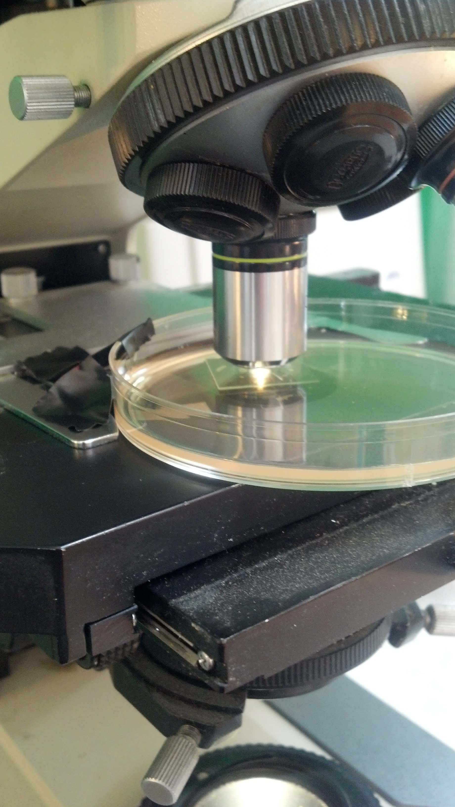
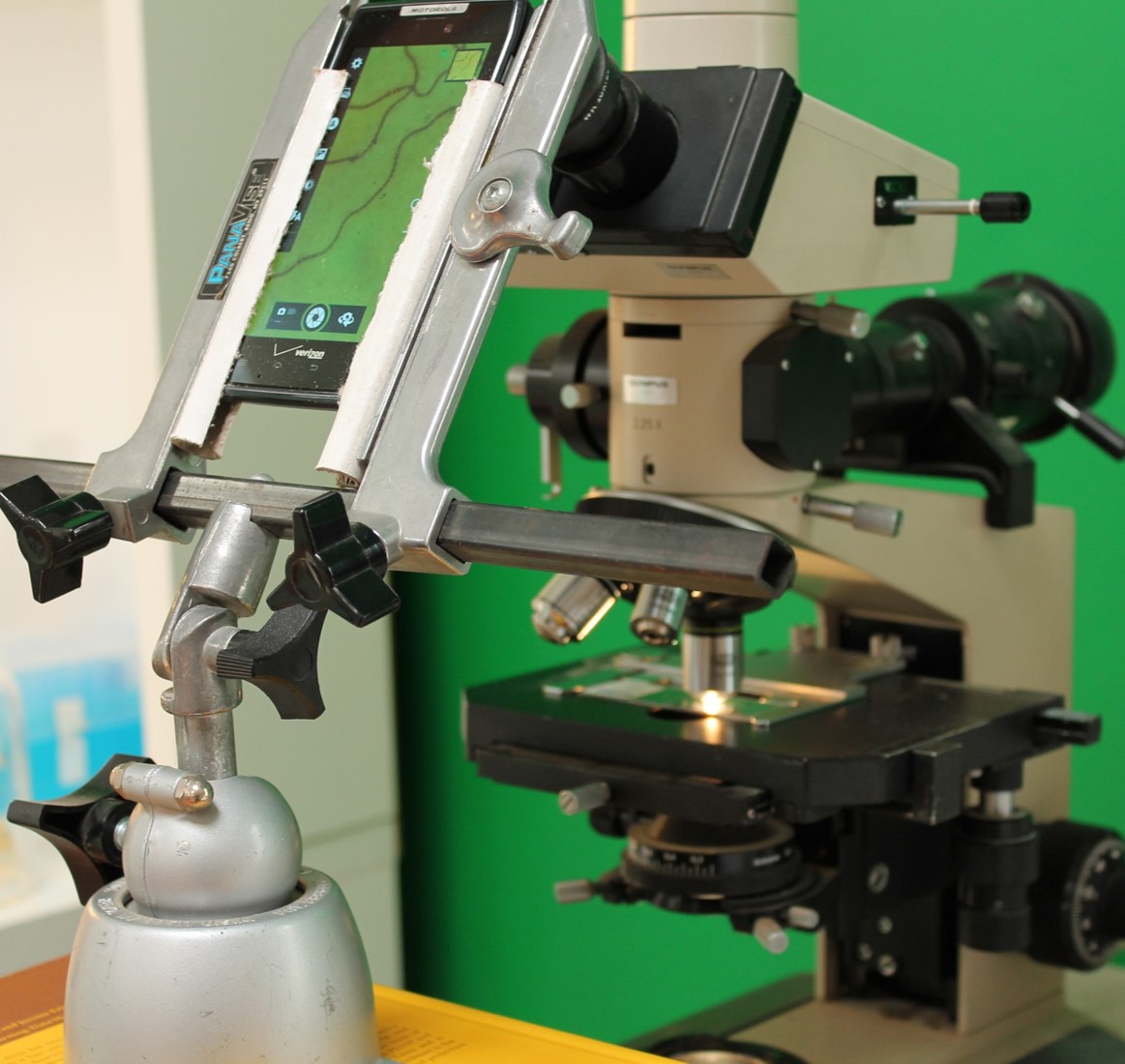
BOSSlab's research microscope panning over agar dish
Hardware Components
This is how data collection works. Ultimately, a raspberry pi controller should continuously pan across the dish, capturing a "googleMaps-like" collection of tile images. like this http://www.illustris-project.org/explorer/
Images -> Data
The goal is to take pictures below and use image processing to output results: mainly distinguish between two types of cells: vegetative and heterocyst.
These guys organize in a pattern that forms naturally in the simplest organisms - cyanobacteria. We know how to add DNA to bacteria, so can we engineer a change in the pattern, and build our own?
The normal form form for data storage goes something like this
Some helpful links for img proc
IPython basics http://nbviewer.ipython.org/github/ipython/ipython/blob/1.x/examples/notebooks/Part%205%20-%20Rich%20Display%20System.ipynb
Skimage basics http://scipy-lectures.github.io/packages/scikit-image/
Demo Code for "Skeleton-ize" method: http://scikit-image.org/docs/dev/auto_examples/plot_medial_transform.html#example-plot-medial-transform-py
Gallery of skimage techniques: http://scikit-image.org/docs/dev/auto_examples/
"Plot-Matching" http://scikit-image.org/docs/dev/auto_examples/plot_matching.html The key to getting aligned tiles (if stepper isn't perfect), we'll match various cells in img(i-d,j) to img(i,j) to determine d