Overview
This week is about getting familiar with networks, and we'll focus on four main elements
- Basic mathematical description of networks
- The
NetworkXlibrary - Matplotlib, binning, and plotting degree distributions
- Random networks
Part 1: Basic mathematical description of networks
This week, let's start with some lecturing. I love networks, so I'll take some time time today to tell you about them.
Video Lecture. Start by watching the "History of Networks".
from IPython.display import YouTubeVideo
YouTubeVideo("qjM9yMarl70",width=800, height=450)
Video Lecture. Then check out a few comments on "Network Notation".
YouTubeVideo("MMziC5xktHs",width=800, height=450)
Reading. We'll be reading the textbook Network Science (NS) by Laszlo Barabasi. You can download the whole thing for free here. You can also download all chapters as a single file
- Read chapter 1.
- Read chapter 2.
Exercises
Chapter 1 (Don't forget that you should be answering these in an IPython notebook.)
- List three different real networks and state the nodes and links for each of them.
- Tell us of the network you are personally most interested in. Address the following questions:
- What are its nodes and links?
- How large is it?
- Can be mapped out?
- Why do you care about it?
- In your view what would be the area where network science could have the biggest impact in the next decade? Explain your answer - and base it on the text in the book.
Chapter 2
- Section 2.5 states that real networks are sparse. Can you think of a real network where each node has many connections? Is that network still sparse? If yes, can you explain why?
There are more questions on Chapter 2 below.
Part 2: The awesome NetworkX library
NetworkX should already be installed as part of your Anaconda Python distribution. But you don't know how to use it yet. The best way to get familiar is to work through a tutorial. That's what the next exercise is about
Exercises:
- Go to the
NetworkXproject's tutorial page. The goal of this exercise is to create your ownnotebookthat contains the entire tutorial. You're free to add your own (e.g. shorter) comments in place of the ones in the official tutorial - and change the code to make it your own where ever it makes sense.- Go to NS Section 2.12: Homework, then
- Write the solution exercise 2.1 (the 'Königsberg Problem') from NS in your
notebook.- Solve exercise 2.3 ('Graph representation') from NS using
NetworkXin yournotebook. (You don't have to solve the last sub-question about cycles of length 4 ... but I'll be impressed if you do it).- Solve exercise 2.5 ('Bipartite Networks') from NS using
NetworkXin yournotebook.
Video Lecture: Once again, it's time to stop working for a couple of minutes to hear me talk about plotting with
NetworkX.
YouTubeVideo("iDlb9On_TDQ",width=800, height=450)
Part 3: Plotting degree distributions
As always we'll learn about degree-distribution plotting by creating a notebook and trying it out.
Exercises:
Begin by importing the right packages. Start by importing
matplotlib.pyplot(for plotting),numpy(for binning and other stuff),random(for generating random numbers), andnetworkx(for generating networks.)
- Binning real numbers
- Let's do a gentle start and use the
randomlibrary generate 5000 data points from a Gaussian distribution with $\mu = 2$ and $\sigma = 0.125$.- Now, let's use
numpy.histogramto bin those number into 10 bins. What does thenumpy.histogramfunction return? Do the two arrays have the same length?- Then we use
matplotlib.pyplot.plotto plot the binned data. You will have to deal with the fact that the counts- and bin-arrays have different lengths. Explain how you deal with this problem and why.- Binning integers
- But binning real numbers into a fixed number of bins is easy when
numpy.histogramdoes all the work and finds the right bin boundaries for you.Now we'll generate a bunch of integers and set the bin boundaries manually. This time, let's grab data from a Poisson distribution. As it turns out
numpyalso has some convenient random number generators. Usenumpy.random.poissonto generate 5000 numbers drawn from a Poisson distribution characterized by $\lambda = 10$. Find the maximum and minimum value of your 5000 random numbers.
- Instead of simplify specifying the number of bins for
numpy.histogram, let's specify the bins we want using a vector.Create a vector $v$ that results in a binning that puts each integer value in its own bin and where the first bin contains the minimum number you found above, and the last bin contains the maximum number. Use the vector by setting
numpy.histogram'sbinparameter asbin =$v$. What is the sum over bin counts? Explain how the binning-vectors first and last element relates to the min and max from the Poisson distribution.
- Now, use a bar chart (
matplotlib.pyplot.bar) to plot the distribution- Binning and plotting degree distributions.
- Let's generate the Erdös-Renyi (ER) network which has a degree distribution that matches the Poisson distribution above.
First we have to figure out which values the ER parameters (N and p) should assume. It's easy to see that $N = 5000$, but how do you find $p$? Hint: The parameter $\lambda$ in the Poisson distribution corresponds to the average degree, so you have to find a $p$ that results in an average degree, $k = 10$. And you know that $\langle k \rangle = p (N-1)$, which will give you $p$. Note that Python by default returns the result of divisions as the most precise of the datatypes involved (for instance, try computing
1/2and1.0/2.0in your notebook). If you want division to always give you a decimal number, you can enterfrom __future__ import divisionat the beginning of your notebook.
- Now, use
networkxto create the graph and extract the degree distribution.- Finally, create a nice bar plot of the degree distribution, including axes labels and a plot title. Make sure that it looks like the Poisson distribution you plotted above.
Part 4: Random networks
Video Lecture. Now it's time to relax and watch a few minutes of info on Random Networks.
YouTubeVideo("c_SbQCzgqb0",width=800, height=450)
Reading. Read section 3.1-3.7 (the most important part is 3.1-3.4) of Chapter 3 of Network Science. You can find the entire book here.
Exercises (should be completed in a
notebook):
- Work through NS exercise 3.1 ('Erdős-Rényi Networks'). The exercise can be found in Section 3.11: Homework.
- Paths. Plot a random network with 200 nodes and an average degree of 1.5. (I suggest using
networkx.drawand reading the documentation carefully to get an overview of all the options and what they look like. For example, you may want to shrink the node size).
- Extract the Giant Connected Component, GCC. (Hint. You can use
networkx.connected_component_subgraphs)- Choose a node at random from the GCC. (Hint: You may want to try
random.choice.)- Find all nodes that are precisely 2 steps away from that node. (Hint. I suggest
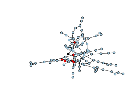
networkx.single_source_shortest_path_length)- Plot the GCC with the following choice of colors. Starting node black (
"#000000"). The nodes 2 steps away red ("#ff0000"). All other nodes blue ("#A0CBE2"). Again, I suggest usingnetworkx.draw()and reading the documentation carefully find out how to color individual nodes.