Realization of Recursive Filters
This jupyter notebook is part of a collection of notebooks on various topics of Digital Signal Processing. Please direct questions and suggestions to Sascha.Spors@uni-rostock.de.
Direct Form Structures
The output signal $y[k] = \mathcal{H} \{ x[k] \}$ of a recursive linear-time invariant (LTI) system is given by
\begin{equation} y[k] = \frac{1}{a_0} \left( \sum_{m=0}^{M} b_m \; x[k-m] - \sum_{n=1}^{N} a_n \; y[k-n] \right) \end{equation}where $a_n$ and $b_m$ denote constant coefficients and $N$ the order. Note that systems with $M > N$ are in general not stable. The computational realization of above equation requires additions, multiplications, the actual and past samples of the input signal $x[k]$, and the past samples of the output signal $y[k]$. Technically this can be realized by
- adders
- multipliers, and
- unit delays or storage elements.
These can be arranged in different topologies. A certain class of structures, which is introduced in the following, is known as direct form structures. Other known forms are for instance cascaded sections, parallel sections, lattice structures and state-space structures.
For the following it is assumed that $a_0 = 1$. This can be achieved for instance by dividing the remaining coefficients by $a_0$.
Direct Form I
The direct form I is derived by rearranging above equation for $a_0 = 1$
\begin{equation} y[k] = \sum_{m=0}^{M} b_m \; x[k-m] + \sum_{n=1}^{N} - a_n \; y[k-n] \end{equation}It is now evident that we can realize the recursive filter by a superposition of a non-recursive and a recursive part. With the elements given above, this results in the following block-diagram
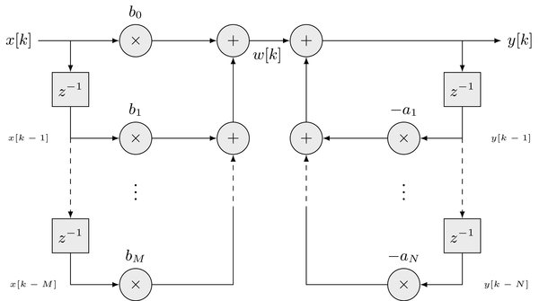
This representation is not canonical since $N + M$ unit delays are required to realize a system of order $N$. A benefit of the direct form I is that there is essentially only one summation point which has to be taken care of when considering quantized variables and overflow. The output signal $y[k]$ for the direct form I is computed by realizing above equation.
The block diagram of the direct form I can be interpreted as the cascade of two systems. Denoting the signal in between both as $w[k]$ and discarding initial values we get
\begin{align} w[k] &= \sum_{m=0}^{M} b_m \; x[k-m] = h_1[k] * x[k] \\ y[k] &= w[k] + \sum_{n=1}^{N} - a_n \; w[k-n] = h_2[k] * w[k] = h_2[k] * h_1[k] * x[k] \end{align}where $h_1[k] = [b_0, b_1, \dots, b_M]$ denotes the impulse response of the non-recursive part and $h_2[k] = [1, -a_1, \dots, -a_N]$ for the recursive part. From the last equality of the second equation and the commutativity of the convolution it becomes clear that the order of the cascade can be exchanged.
Direct Form II
The direct form II is yielded by exchanging the two systems in above block diagram and noticing that there are two parallel columns of delays which can be combined, since they are redundant. For $N=M$ it is given as
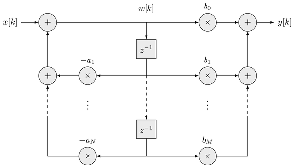
Other cases with $N \neq M$ can be considered for by setting coefficients to zero. This form is a canonical structure since it only requires $N$ unit delays for a recursive filter of order $N$. The output signal $y[k]$ for the direct form II is computed by the following equations
\begin{align} w[k] &= x[k] + \sum_{n=1}^{N} - a_n \; w[k-n] \\ y[k] &= \sum_{m=0}^{M} b_m \; w[k-m] \end{align}The samples $w[k-m]$ are termed state (variables) of a digital filter.
Transposed Direct Form II
The block diagrams above can be interpreted as linear signal flow graphs. The theory of these graphs provides useful transformations into different forms which preserve the overall transfer function. Of special interest is the transposition or reversal of a graph which can be achieved by
- exchanging in- and output,
- exchanging signal split and summation points, and
- reversing the directions of the signal flows.
Applying this procedure to the direct form II shown above for $N=M$ yields the transposed direct form II
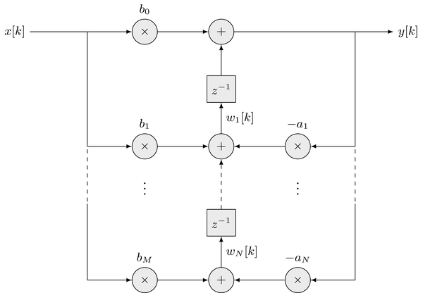
The output signal of the transposed direct form II is given as
\begin{equation} y[k] = b_0 x[k] + \sum_{m=1}^{M} b_m x[k-n] - \sum_{n=1}^{N} a_n y[k-n] \end{equation}Using the signal before the $n$-th delay unit as internal state $w_n[k]$ we can reformulate this into a set of difference equations for computation of the output signal
\begin{align} w_n[k] &= \begin{cases} w_{n+1}[k-1] - a_n y[k] + b_n x[k] & \text{for } n=0,1,\dots,N-1 \\ -a_N y[k] + b_N x[k] & \text{for } n=N \end{cases}\\ y[k] &= w_1[k-1] + b_0 x[k] \end{align}Example - Computation of output signal
The following example illustrates the computation of the impulse response $h[k]$ of a 2nd-order recursive system using the transposed direct form II as realized by scipy.signal.lfilter.
import numpy as np
import matplotlib.pyplot as plt
import scipy.signal as sig

p = 0.90 * np.exp(-1j * np.pi / 4)
a = np.poly([p, np.conj(p)])  # denominator coefficients
b = [1, 0, 0]  # numerator coefficients
N = 40  # number of computed samples

# generate input signal (= Dirac impulse)
k = np.arange(N)
x = np.where(k == 0, 1.0, 0.0)

# filter signal using transposed direct form II
h = sig.lfilter(b, a, x)

# plot output signal
plt.figure(figsize=(8, 4))
plt.stem(h)
plt.title("Impulse response")
plt.xlabel(r"$k$")
plt.ylabel(r"$h[k]$")
plt.axis([-1, N, -1.5, 1.5])
plt.grid()
Exercise
- Compute the step-response $h_\epsilon[k] = \mathcal{H} \{ \epsilon[k] \}$ of the filter by modifying above example.
Solution: The step response can be computed by changing the input signal to
x = np.where(k>=0, 1.0, 0.0)
or by cumulative summation of the impulse response due to the relation $h_\epsilon[k] = \sum_{\kappa =0}^k h[k]$ of the step response to the impulse response
he = np.cumsum(h)
Copyright
This notebook is provided as Open Educational Resource. Feel free to use the notebook for your own purposes. The text is licensed under Creative Commons Attribution 4.0, the code of the IPython examples under the MIT license. Please attribute the work as follows: Sascha Spors, Digital Signal Processing - Lecture notes featuring computational examples.