Notebook

Ch2. Linear Regression¶

Overview¶

[TOC]

Simple linear regression
Evaluating the model
Multiple linear regression
Polynomial regression
Regularization
Applying linear regression
Fitting models with gradient descent
Summary

Simple Linear Regression¶

Training Data (학습 데이터)¶

used to estimate the parameters of a model.
past observations of explanatory variables + respose variables
cf. explanatory variable aka independent variable (독립 변수, 설명 변수)
cf. response variable aka dependent variable (반응 변수, 종속 변수)

Prediction (using model) (예측)¶

using explanatory variables (that have not been previously observes)
estimate response variable

Goal in Regression Problem:¶

predict the value of a continuous response variable

Simple Linear Regression (단순 선형회귀)¶

linear relationship betw. 1 response variable and 1 explanatory variable

Ex: Pizza¶

In [1]:

import matplotlib.pyplot as plt
X = [[6], [8], [10], [14],   [18]]
y = [[7], [9], [13], [17.5], [18]]
plt.figure()
plt.title('Pizza price plotted against diameter')
plt.xlabel('Diameter in inches')
plt.ylabel('Price in dollars')
plt.plot(X, y, 'k.')
plt.axis([0, 25, 0, 25])
plt.grid(True)
plt.show()

Actual Linear Regression Example¶

In [2]:

from sklearn.linear_model import LinearRegression
# Training data
X = [[6], [8], [10], [14],   [18]]
y = [[7], [9], [13], [17.5], [18]]
# Create and fit the model
model = LinearRegression()
model.fit(X, y)
print 'A 12" pizza should cost: $%.2f' % model.predict([12])[0]

A 12" pizza should cost: $13.68

Hyperplane¶

assumption: linear relationship exists betw. response var. and explanatory var.
this relationship is modeled as a linear surface, hyperplane
subspace that's 1 dim. less than the ambient space that contains it

Estimator (예측 규칙, 예측 모델?)¶

eg: sklearn.linear_model.LinearRegression class
predicts a value based on the observed data
important methods (all estimator implements)

name	role
`fit()`	learns the parameters of a model
`predict()`	predicts the value of response variable, using learned parameters

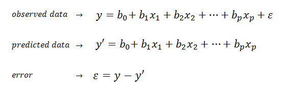
    y = α + βx

name	desc.
y	predicted value of the response var.
x	explanatory variable
α,β	intercept term / coefficient - paramters of the model (learned by the learning algorithm)

In [3]:

plt.xlabel('Diameter in inches'); plt.ylabel('Price in dollars');
X2 = [[0], [10], [14], [25]]
plt.plot(X2, model.predict(X2), color='blue', linewidth=2)
plt.plot(X,y, 'k.')
plt.grid(True)
plt.show()

Ordinary Least Squares (or Linear Least Squares)¶

want to find model that produces the best fitting model

model that fits the training data

Evaluating the fitness of a model with a cost function¶

what's criteria for best-fitting regression?

Cost Function (aka Loss Function)¶

Used to define & measure the error (오차) of a model

residual (or training error, 잔차): differences betw. predicted values & observed values in the training set
prediction error / test error: diff. in the test set

Residual sum of squares cost function

In [4]:

import numpy as np
print "Residual sum of squares: %.2f" % np.mean((model.predict(X) - y) ** 2)

Residual sum of squares: 1.75

Solving ordinary least squares (최소 자승) for simple linear regression¶

1) solve β: calculate variance (분산) & covariance (공분산) of x¶

β = cov(x,y) / var(x)

2) solve α: calculate using means of x,y and β¶

α = mean(y) - β mean(x)

Evaluating the Model¶

r-squared¶

how well the observed values of the response variables are predicted by the model

proportion of the variance in the response variable that is explaned by the model

In [5]:

from sklearn.linear_model import LinearRegression

X = [[6], [8], [10], [14], [18]]; y = [[7], [9], [13], [17.5], [18]]
X_test = [[8],  [9],  [11], [16], [12]]; y_test = [[11], [8.5], [15], [18], [11]]

model = LinearRegression()
model.fit(X, y)
print 'R-squared: %.4f' % model.score(X_test, y_test)

R-squared: 0.6620

Multiple Linear Regiression¶

Formal Definition¶

multiple linear regression uses a coefficient for each of an arbitrary number of explanatory variables

in matrix form:

estimation of β (using matrix notation)¶

In [6]:

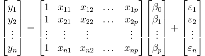
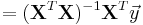
from numpy.linalg import inv; from numpy import dot, transpose
X = [[1, 6, 2], [1, 8, 1], [1, 10, 0], [1, 14, 2], [1, 18, 0]]; y = [[7],    [9],    [13],    [17.5],  [18]]
print dot(inv(dot(transpose(X), X)), dot(transpose(X), y))

[[ 1.1875    ]
 [ 1.01041667]
 [ 0.39583333]]

or, use least square function that NumPy provides:

In [7]:

from numpy.linalg import lstsq
print lstsq(X, y)[0]

[[ 1.1875    ]
 [ 1.01041667]
 [ 0.39583333]]

Let's predict y (with second explanatory variable)!

In [8]:

X = [[6, 2], [8, 1], [10, 0], [14, 2], [18, 0]]; y = [[7],    [9],    [13],    [17.5],  [18]]
model = LinearRegression()
model.fit(X, y)
X_test = [[8, 2], [9, 0], [11, 2], [16, 2], [12, 0]]; y_test = [[11],   [8.5],  [15],    [18],    [11]]
predictions = model.predict(X_test)

for i, prediction in enumerate(predictions):
	print 'Predicted: %s, Target: %s' % (prediction, y_test[i])
print 'R-squared: %.2f' % model.score(X_test, y_test)

Predicted: [ 10.0625], Target: [11]
Predicted: [ 10.28125], Target: [8.5]
Predicted: [ 13.09375], Target: [15]
Predicted: [ 18.14583333], Target: [18]
Predicted: [ 13.3125], Target: [11]
R-squared: 0.77

Analysis¶

additional explanatory variable improved the performance of the model
multiple linear regression model performs significantly better than the simple LR model.

Polynomial Regression¶

Quadratic Regression¶

cf. PolynomialFeatures transformer can be used to add polynomial features to a feature representation

cf. Feature: tuple of explanatory variables

In [9]:

import numpy as np
import matplotlib.pyplot as plt
from sklearn.linear_model import LinearRegression
from sklearn.preprocessing import PolynomialFeatures

X_train = [[6], [8], [10], [14], [18]]
y_train = [[7],    [9],    [13],    [17.5],  [18]]
X_test = [[6],  [8],   [11], [16]]
y_test = [[8],   [12],  [15], [18]]

regressor = LinearRegression()
regressor.fit(X_train, y_train)
xx = np.linspace(0, 26, 100)
yy = regressor.predict(xx.reshape(xx.shape[0], 1))
plt.plot(xx, yy)

featurizer = PolynomialFeatures(degree=2)
X_train_quad = featurizer.fit_transform(X_train)
X_test_quad = featurizer.transform(X_test)

regressor_quad = LinearRegression()
regressor_quad.fit(X_train_quad, y_train)
xx_quad = featurizer.transform(xx.reshape(xx.shape[0], 1))

plt.plot(xx, regressor_quad.predict(xx_quad), c='r', linestyle='--')
plt.title('Pizza price regressed on diameter (linear, quadratic)')
plt.xlabel('Diameter in inches')
plt.ylabel('Price in dollars')
plt.axis([0, 25, 0, 25])
plt.grid(True)
plt.scatter(X_train, y_train)
plt.show()

print X_train
print X_train_quad
print X_test
print X_test_quad

print 'Simple LR R^2', regressor.score(X_test, y_test)
print 'Quadratic Regression R^2', regressor_quad.score(X_test_quad, y_test)

[[6], [8], [10], [14], [18]]
[[  1   6  36]
 [  1   8  64]
 [  1  10 100]
 [  1  14 196]
 [  1  18 324]]
[[6], [8], [11], [16]]
[[  1   6  36]
 [  1   8  64]
 [  1  11 121]
 [  1  16 256]]
Simple LR R^2 0.809726797708
Quadratic Regression R^2 0.867544365635

Overfitting (과적합)¶

instead of induce a general rule,
memorized the inputs and outputs from the training data
so performs poorly on test data

Overfitting and Underfitting¶

overfit_underfit

Regularization¶

Collection of techniques that can be used to prevent overfitting

Penalty against complexity

Ridge Regression¶

using L2 norm of the coefficients

Least Absolute Shrinkage and Selection Operator (LASSO)¶

using L1 norm of the coefficients

Elastic Net Regularization¶

linearly combines L1 and L2 penalties(norms)

Applying LR¶

In [10]:

import pandas as pd
df = pd.read_csv('/Users/apollos/Desktop/Python/scikit-learn/winequality-red.csv', sep=';') 
df.describe()

import matplotlib.pylab as plt
plt.scatter(df['alcohol'], df['quality'])
plt.xlabel('Alcohol')
plt.ylabel('Quality')
plt.title('Alcohol Against Quality')
plt.show()

from sklearn.linear_model import LinearRegression
import pandas as pd
import matplotlib.pylab as plt
from sklearn.cross_validation import train_test_split

df = pd.read_csv('/Users/apollos/Desktop/Python/scikit-learn/winequality-red.csv', sep=';')
X = df[list(df.columns)[:-1]]
y = df['quality']
X_train, X_test, y_train, y_test = train_test_split(X, y)

regressor = LinearRegression()
regressor.fit(X_train, y_train)
y_predictions = regressor.predict(X_test)
print 'R-squared:', regressor.score(X_test, y_test)

/Users/apollos/Library/Enthought/Canopy_64bit/User/lib/python2.7/site-packages/pandas/io/excel.py:626: UserWarning: Installed openpyxl is not supported at this time. Use >=1.6.1 and <2.0.0.
  .format(openpyxl_compat.start_ver, openpyxl_compat.stop_ver))

R-squared: 0.333280171254

Fitting Models with Gradient Descent¶

Gradient Descent¶

an optimization algorithm that can be used to estimate the local minimum of a function

learning rate : controls the size of the steps

too small: too long time for convergence
too large: overstepping -> could oscillate around the optimal values

type	training data coverage	result
Batch GD	all	deterministic
Stochastic GD (SGD)	one / iteration	random

In [11]:

import numpy as np
import random
from sklearn.datasets import load_boston
from sklearn.linear_model import SGDRegressor
from sklearn.cross_validation import cross_val_score
from sklearn.preprocessing import StandardScaler
from sklearn.cross_validation import train_test_split

data = load_boston()
X_train, X_test, y_train, y_test = train_test_split(data.data, data.target)
print 'length of training set: ', len(y_train)
print 'length of test set: ', len(y_test) # train:test = 3:1
# random.seed(len(y_train))
X_scaler = StandardScaler()
y_scaler = StandardScaler()
X_train = X_scaler.fit_transform(X_train)
y_train = y_scaler.fit_transform(y_train)
X_test = X_scaler.transform(X_test)
y_test = y_scaler.transform(y_test)

regressor = SGDRegressor(loss='squared_loss')
scores = cross_val_score(regressor, X_train, y_train, cv=5)
print 'Cross validation r-sqaured scores:', scores
print 'Average cross validation r-squared score:', np.mean(scores)
regressor.fit_transform(X_train, y_train)
print 'Test set r-squared score', regressor.score(X_test, y_test)

length of training set:  379
length of test set:  127
Cross validation r-sqaured scores: [ 0.56648863  0.6538719   0.69710693  0.7509363   0.62969822]
Average cross validation r-squared score: 0.659620397034
Test set r-squared score 0.75891216356

Summary¶

3 Cases of LR¶

Simple LR
Multiple LR
Polynomial Regression

Generalized Linear Model¶

framework for modeling linear relationships

How to minimize cost function (solve the model, find parameters, ...)¶

solve analytically (using Linear Algebra)
use gradient descent

Next Chapter¶

how to create features for different types of explanatory variables
especially, categorical variables, texts, images