Interpolating a function via circular arcs in Julia
Time for some recreational math.
Let's try and write a program, which given a function equation and a segment, for example:
would build an approximation of this with a sequence of circular arcs.
As a bonus, we would like to generate the corresponding G-codes for these arcs, so the output of our program could be fed to some automatic cutting tool, which would cut out a nice parabola, so we could make a pendant, put it on the neck and proudly wear as a proof of our accomplishments!
Possible solution
Given that the problem has real-world practical applications (in 3D printing, machining et al), there has been a wealth of research on the topic.
I've taken this ancient thesis as a starting point, mostly because of the simplicity of the approach it is taking.
So what we are going to try is essentially a rather brute force, greedy algorithm.
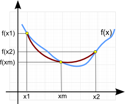
For some given segment [x1, x2], we draw the arc approximation as a circle, that passes through the point (x1, f(x1)), the point (x2, f(x2)) and also the third, middle point (xm, f(xm)), which for simplicity we can assume is equidistant from x1 and x2:
Then the algorithm proceeds as following:
- Start from trying to fit an arc to the whole segment [a, b] (so that x1=a and x2=b) and compute the error value
- If error is good enough then we are done, otherwise we shrink the current segment by some ratio (say, 0.8), such that point x1 stays in place and point x2 moves left, repeating this until the error is good enough
- Once the current arc is fit, we repeat the same thing with the next one, this time trying to cover the remaining part of the segment (i.e. x1=x2_prev and x2=b)
- The previous two steps get repeated until we cover the whole segment (so that x2=b and the error is good enough)
Essentially, we will try packing the arcs left-to-right, in a "greedy" way, until the whole segment is covered.
Julia language
Why using Julia programming language in particular?.. This sums it up nicely.
Matlab has established itself as a de-facto standard tool for scientific computations. I've been using it almost daily at the job, and it's rather good at what it does.
It also has flaws:
- Too expensive
- Too slow, in general
- The programming language itself is not very expressive
The first problem is what Octave is trying to solve, by being free and trying to replicate most of the Matlab's functionality. However, it's even "slower" than Matlab, and the language itself is pretty much the same, except of a few improvements (which was their goal, to start with).
The second problem can be somewhat mitigated in Matlab itself via vectorization (i.e. operate on the level of whole vectors/matrices as opposed to separate elements) or re-implementing performance-critical parts in C/C++.
The third one is something that just had to be lived with - Matlab was apparently designed as BASIC for engineers, as simple and straightforward imperative/array programming language as possible. Which is both a benefit and a flaw.
Julia is trying to solve the mentioned problems, and some others. At the moment of writing the current stable version is 0.35 (and 0.4 is being in the works), which suggests that there is still a way to go until it can be considered a mature and stable tool.
But even now it seems to be doing quite a good job.
And unlike Matlab, it's fun to program with, especially using a pimped REPL like IJulia. In fact, this article is just an IJulia notebook, which is available here. So let's go step-by-step and implement the building blocks that we need for the algorithm to run.
Circle through three points
The basic operation we need first is finding a circle that goes through the three given points. There does noes not seem a corresponding library/function available in Julia yet, so let's roll our own, having looked into the Wikipedia article.
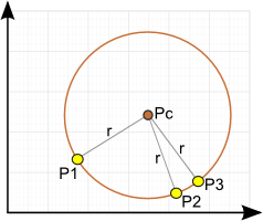
Given any three points P1, P2 and P3 we can find the circle with center Pc and radius r, circumscribed over these points using the following formulas (this is just an one of the possible forms of equations):
Unit testing
But before writing any Julia code let's first figure out how could we test it.
There is a Base.Test Julia module which we can include and perform some basic unit testing:
using Base.Test

@test 1 + 2 == 3
The test passes fine, there is no complaints. Let's try another one:
@test .1 + .2 == .3
test failed: 0.1 + 0.2 == 0.3
while loading In[2], in expression starting on line 1

 in error at error.jl:21 (repeats 2 times)
As you can see, this one fails. Why?.. Well, simply because 0.1 plus 0.2 is not equal 0.3.
Here's a better way:
@test_approx_eq (.1 + .2) .3
Now it passes alright. What if we wanted to compare tuples?
@test_approx_eq (1 + 2, .1 + .2) (3, .3)
`full` has no method matching full(::(Int64,Float64))
while loading In[4], in expression starting on line 1

 in test_approx_eq at test.jl:88
 in test_approx_eq at test.jl:119
This does not work, unfortunately, but Julia's flexible enough, so we can fix it by rolling our own unit testing macro, with Blackjack and stuff:
is_close(x::Number, y::Number, epsilon = eps()) =
    abs(y - x) <= max(1, abs(x), abs(y))*epsilon

is_close(x, y, epsilon = eps()) =
    all(x -> is_close(x..., epsilon), zip(x, y))

function test_close(a, b, eps, astr, bstr)
    if !is_close(a, b, eps)
        println("test failed: $(astr) is not close to $(bstr);\n   $(a) vs $(b)")
    end
end

macro test_close(a, b)
    :( test_close($(a), $(b), 1e-6, $(string(a)), $(string(b))) )
end

@test_close (1 + 2, .1 + .2) (3, .3)
@test_close (1 + 2, .1 + .2) (2, .3)
test failed: (1 + 2,0.1 + 0.2) is not close to (2,0.3);
   (3,0.30000000000000004) vs (2,0.3)
There is a bunch of language concepts already packed in a few lines here, such as function overloading/specialization, default parameter values, type inference, iterators, lambdas, tuple splicing, string interpolation, macros and what have you.
But this is just a glimpse into the Julia's capabilities, so if it does not make sense to you, then let's just pretend that Julia's test library already has it and move on.
Circle through three points - the code
Armed with this, we can finally write some code, related to the problem at hand (and the corresponding unit tests). It is a rather straightforward translation of the formulas:
# returns the (center, radius) of the circle, circumscribed around three points
function circumscribed_circle(P1, P2, P3)
    d12 = vec(P1 - P2); n12 = dot(d12, d12)
    d23 = vec(P2 - P3); n23 = dot(d23, d23)
    d31 = vec(P3 - P1); n31 = dot(d31, d31)
    d = norm(cross([d12; 0], [d23; 0]))
    r = sqrt(n12*n23*n31)/(2d)
    alpha = n23*dot(d12, d31)
    beta = n31*dot(d12, d23)
    gamma = n12*dot(d31, d23)
    Pc = -(alpha*P1 + beta*P2 + gamma*P3)/(2d^2)
    (Pc, r)
end

# the circumscribed_circle tests
@test_close ([-1, 1], 1) circumscribed_circle([-2; 1], [-1; 2], [0; 1])
@test_close ([0, 0], 2) circumscribed_circle([2; 0], [0; 2], [sqrt(2); sqrt(2)])
Point orientation
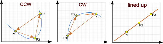
Another function we'll need is the one that finds out whether three points are winded counter-clockwise (CW) or clock-wise.
We can do that by looking at the sign of the third component of a vector cross product between two vectors spanning our three points.
As a bonus we can also determine if all the three points are lined up (i.e they are neither CW nor CCW oriented).
const EPSILON = 1e-5

# finds the orientation of three 2D points
# -1 for CW, 1 for CCW, 0 if on the same line
function orientation(P1, P2, P3)
    _, _, cz = cross([vec(P2 - P1); 0], [vec(P3 - P1); 0])
    if abs(cz) < EPSILON
        cz = 0
    end
    sign(cz)
end

@test 1 == orientation([0; 0], [1; 0], [2; 2])
@test 0 == orientation([0; 0], [1; 1], [2; 2])
@test -1 == orientation([0; 0], [2; 2], [1; 0])
Handling three points on the same line
Now that we've got our circumscribed circle function, let's try some other point combination:
circumscribed_circle([1; 1], [2; 2], [3; 3])
([NaN,NaN],Inf)
Oops.
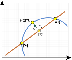
Apparently, the part with "any" three points was not quite correct: we can't make an arc through them if they happen to be on the same line. Since the problem constraint was to use only arc primitives (even though in practice G-codes do allow straight line segments as well), we'd need to remedy it somehow.
A solution is to offset the middle point somewhat in the direction, orthogonal to the line in question:
The corresponding formulas and the code:
function offset_orthogonal(P2, P3)
    D = P2 - P3
    Dp = [-D[2]; D[1]]
    P2 + EPSILON*Dp/norm(Dp)
end

@test 0 != orientation([0; 0], offset_orthogonal([1; 1], [2; 2]), [2; 2])
Arc equation
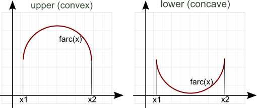
What we are going to do, essentially, is to split the function's range into segments and on each segment approximate it with another function (of an arc). The arc function looks like following (coming from the circle equation):
There are two possibilities for the arc function: it can be either convex or concave, which corresponds to the +/- in the equation:
The code:
function f_arc(x, c, R, convex = true)
    cx, cy = c
    plusminus = convex ? 1 : -1
    cy + plusminus*sqrt(max(0, R^2 - (x - cx)^2))
end

@test_close 3 f_arc(1, [1; 1], 2, true)
@test_close -1 f_arc(1, [1; 1], 2, false)

@test_close 1 f_arc(3, [1; 1], 2, true)
@test_close 1 f_arc(3, [1; 1], 2, false)
Arc data structure
To describe an arc segment it's convenient to group several attributes into a dedicated data structure. In Julia it's defined as following:
type ArcSeg
    c::Array{Float64, 1}  # arc center
    R::Float64            # arc radius
    a::Float64            # segment start
    b::Float64            # segment end
    convex::Bool          # true if top part of the circle (otherwise concave)
    m::Float64            # middle point ratio
end
We have field data types specified here explicitly, but generally Julia does not require that.
Making an arc
Here's a function to actually draw an arc through two corner points and the middle one, given the function and the segment:
# makes an arc going through the segment ends
function make_arc(f, seg, middle_ratio = 0.5)
    a, b = seg
    m = a + (b - a)*middle_ratio
    pa, pb, pm = [a; f(a)], [b; f(b)], [m; f(m)]
    # handle the case when all three points are on the same line
    porient = orientation(pa, pm, pb)
    if porient == 0
        # points are on the same line
        pm = offset_orthogonal(pm, pb)
    end
    c, R = circumscribed_circle(pa, pm, pb)
    ArcSeg(c, R, a, b, porient < 0, middle_ratio)
end

#  inscribe an arc into itself
_arc = make_arc(x -> f_arc(x, [1; 1], 5, true), (3, 4), 0.2)
@test_close [1; 1] _arc.c
@test_close (5, 3, 4, 0.2) (_arc.R, _arc.a, _arc.b, _arc.m)
@test _arc.convex
Error metric
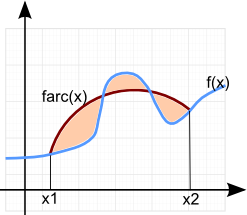
For measuring how far away is our arc from the actual function, we'll use the so-called L1-metric distance between functions:
Essentially, it's the area of undesired "slack" between two curves:
To find the total error on the segment, we need to integrate this distance function (which looks like camel humps in our case):
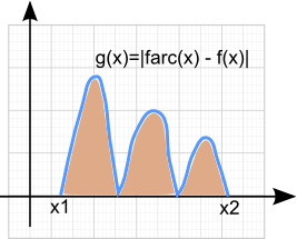
Finding this integral can be done in different ways, but we'll use a rather simple one, trapezoidal integration, whereas the segment is split into a number of chunks of equal width, and the total area is computed as the sum of the corresponding trapezoids:
const NUM_INTEGRATION_SAMPLES = 1000
function integrate_trapezoidal(f, x1, x2, N = NUM_INTEGRATION_SAMPLES)
    @assert(N >= 1)
    dx = (x2 - x1)/N;
    s0 = (f(x1) + f(x2))/2
    (s0 + sum([f(clamp(x1 + i*dx, x1, x2)) for i in 1:(N - 1)]))*(x2 - x1)/N
end

# integrate parabola
@test_close 2^3/3 integrate_trapezoidal(x -> x^2, 0, 2)
@test_close 2^3/3 integrate_trapezoidal(x -> x^2, 0, 2, 10000)
@test_close 2^3/3 integrate_trapezoidal(x -> x^2, 0, 2, 1000000)

# integrate half a circle (offset by 1 upwards from X axis)
@test_close (pi*3^2/2 + 3*2) integrate_trapezoidal(x -> f_arc(x, [1; 1], 3, true), 1 - 3, 1 + 3, 10000)
Then the error function itself is:
function err(f, arc::ArcSeg)
    err_metric(x) = abs(f(x) - f_arc(x, arc.c, arc.R, arc.convex))
    res = integrate_trapezoidal(err_metric, arc.a, arc.b)
end

f(x) = 2
@test is_close(2 - pi/2, err(f, ArcSeg([1; 1], 1, 0, 2, true, 0.1)), 1e-4)
Note that package "Calculus" does have some numerical integration routines, which we could theoretically use, and that's what I tried at first.
That did not work out very well, though. The default integration method (Simpson's) does not seem to converge for some functions.
Another method there is Monte-Carlo integration:
using Calculus
function err_old(f, arc::ArcSeg)
    err_metric(x) = abs(f(x) - f_arc(x, arc.c, arc.R, arc.convex))
    res = Calculus.monte_carlo(err_metric, arc.a, arc.b, NUM_INTEGRATION_SAMPLES)
end

@test_close (2 - pi/2) err_old(f, ArcSeg([1; 1], 1, 0, 2, true, 0.1))
test failed: 2 - pi / 2 is not close to err_old(f,ArcSeg([1,1],1,0,2,true,0.1));
   0.42920367320510344 vs 0.4484735688613066
@test_close (2 - pi/2) err_old(f, ArcSeg([1; 1], 1, 0, 2, true, 0.1))
test failed: 2 - pi / 2 is not close to err_old(f,ArcSeg([1,1],1,0,2,true,0.1));
   0.42920367320510344 vs 0.4610385490322167
The same test both fails and gives different answers in different runs.
Non-deterministic == not good, so let's stick to our own trapezoidal wheel we've just reinvented.
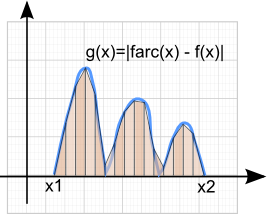
The "ears"
Now, our error metric is still not good enough, since it does not account for certain corner cases ("ears") such as here:
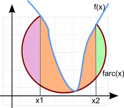
The orange area is the one that we've just computed, but the pink and the green "ears" are the extra pieces that also add to the error value.
Since we generally take three arbitrary points to draw a circle through, such point configuration is not uncommon, and we need to properly adjust the error metric to account for it.
Wikipedia is, again, to the resque for the ears area:
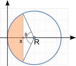
function circle_segment_area(x, R)
    theta = 2acos((R-x)/R)
    R^2*(theta - sin(theta))/2
end

@test_approx_eq circle_segment_area(0, 7) 0
@test_approx_eq circle_segment_area(14, 7) pi*7^2
@test_approx_eq circle_segment_area(7, 7) pi*7^2/2
@test_approx_eq circle_segment_area(2, 7) (pi*7^2 - circle_segment_area(7*2 - 2, 7))
Full error function
Having taken the ears into account, let's write the full error function:
function err1(f, arc::ArcSeg)
    res = err(f, arc)
    # add the "ears" error
    fa, fb = f(arc.a), f(arc.b)
    cx, cy = arc.c[1], arc.c[2]
    if (fa > cy) != arc.convex
        # left "ear"
        res += circle_segment_area(arc.a - (cx - arc.R), arc.R)
    end
    if (fb > cy) != arc.convex
        # right "ear"
        res += circle_segment_area(cx + arc.R - arc.b, arc.R)
    end
    res
end

f(x) = 2
@test is_close(2 - pi/2, err1(f, ArcSeg([1; 1], 1, 0, 2, true, 0.1)), 1e-4)

arc = ArcSeg([1; 1], 1, 0.5, 1.5, true, 0.1)
d = f_arc(0.5, arc.c, arc.R)
f(x) = d
@test is_close(pi - circle_segment_area(d, 1), err1(f, arc), 1e-4)
Fitting a sequence of arcs
Now we put together all the building blocks into the arc fitting procedure, following the steps discussed earlier:
const STEP_RATIO = 0.8
const pick_center_pt = (f, a, b) -> 0.5

function fit_arcs(f, range, tolerance, pick_middle_pt = pick_center_pt)
    ra, rb = range
    D = rb - ra
    rel_tol = tolerance/D
    ca = ra
    arcs = []
    while ca < rb
        cb = rb
        while true
            middle_ratio = pick_middle_pt(f, ca, cb)
            arc = make_arc(f, (ca, cb), middle_ratio)
            E = err1(f, arc)
            if E <= rel_tol*(cb - ca)
                arcs = [arcs, arc]
                ca = cb
                break
            end
            cb = ca + STEP_RATIO*(cb - ca)
        end
    end
    arcs
end
fit_arcs (generic function with 2 methods)
We've left "pick the middle point" as a callback, which by default simply takes the point halfway between the segment ends.
Inspecting the result
We did not write a unit test for this one, since it's a bit too complex of a unit already, but let's try and see how we could test it otherwise.
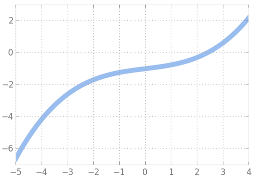
Let's take a simple function as an example:
The Julia's DataFrames library can be used to organize/display the data in tabular form (and do much more than that):
using DataFrames

fmt(x::Float64) = round(x, 3)
fmt(x::Array{Float64,1}) = map(fmt, x)
fmt(x::Bool) = x ? "yes" : "no"
fmt(x) = x

function to_table(arcs)
    DataFrame(
        c = map(x->fmt(x.c), arcs),
        R = map(x->fmt(x.R), arcs),
        a = map(x->fmt(x.a), arcs),
        b = map(x->fmt(x.b), arcs),
        m = map(x->fmt(x.m), arcs),
        convex = map(x->fmt(x.convex), arcs))
end

to_table(fit_arcs(x -> x^3/27 + x/5 - 1, [-5 4], 0.1))
| c | R | a | b | m | convex | |
|---|---|---|---|---|---|---|
| 1 | [11.278,-11.843] | 17.092 | -5.0 | -3.792 | 0.5 | yes |
| 2 | [1.386,-6.401] | 5.805 | -3.792 | -2.158 | 0.5 | yes |
| 3 | [0.554,-5.846] | 4.868 | -2.158 | -0.14 | 0.5 | yes |
| 4 | [-0.888,4.714] | 5.79 | -0.14 | 1.98 | 0.5 | no |
| 5 | [-0.935,3.985] | 5.196 | 1.98 | 3.596 | 0.5 | no |
| 6 | [-5.283,6.839] | 10.391 | 3.596 | 4.0 | 0.5 | no |
It shows us something, but still not much.
Printing G-codes
We can proceed and generate the actual G-codes. The subset that we are interested in is:
G00 X[xpos] Y[ypos] - jump to location xpos, ypos
G02 X[xpos] Y[ypos] I[cdx] J[cdy] - CW rotation ending in location (xpos, ypos), with center relatively offset by (cdx, cdy) from the current location
G02 X[xpos] Y[ypos] R[R] - CW rotation ending in location (xpos, ypos), with radius R from the current location
G03 ... - the same as G02, but for CCW rotation
G02 corresponds to the "convex" arcs, G03 to the "concave" ones.
There are two notations for arc codes: IJ-notation (specifying the relative circle center offset) and R-notation (specifying just the circle radius).
The latter is more compact, but the former is a bit safer, since it potentially allows the controller to do additional consistency checks.
We implement both of them.
function make_g_code(arcs, rformat=true, split_lines=true)
    fmt(x) = (round(x, 3) == round(x, 0)) ? @sprintf("%d", x) : @sprintf("%.3f", x)
    function arc2g(arc)
        a, b = arc.a, arc.b
        fa = f_arc(a, arc.c, arc.R, arc.convex)
        fb = f_arc(b, arc.c, arc.R, arc.convex)
        cx, cy = arc.c
        res = split_lines ? "\n" : ""
        res *= (arc.convex ? "G02" : "G03") * " X$(fmt(b)) Y$(fmt(fb)) "
        res *= rformat ? "R$(fmt(arc.R))" : "I$(fmt(cx - a)) J$(fmt(cy - fa))"
    end
    a1 = arcs[1]
    fa1 = f_arc(a1.a, a1.c, a1.R, a1.convex)
    "G00 X$(fmt(a1.a)) Y$(fmt(fa1)) " * join(map(arc2g, arcs), " ")
end

arc = ArcSeg([1; 1], 1, 0, 2, true, 0.1)
@test "G00 X0 Y1 G02 X2 Y1 R1" == make_g_code([arc], true, false)
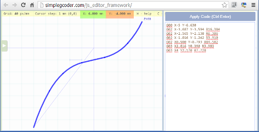
The actual G-codes appearance can be tested online, for example here.
print(make_g_code(fit_arcs(x -> x^3/27 + x/5 - 1, [-5 4], 0.1)))
G00 X-5 Y-6.630
G02 X-3.792 Y-3.778 R17.092
G02 X-2.158 Y-1.804 R5.805
G02 X-0.140 Y-1.028 R4.868
G03 X1.980 Y-0.317 R5.790
G03 X3.596 Y1.441 R5.196
G03 X4 Y2.170 R10.391
Visualization
Let's try and plot the arc approximation ourselves, using whatever facilities Julia provides.
To plot the sequence of arcs, we first need to generate a sequence of corresponding points. For that, let's first write a function "normalize_angle_range", which would arrange two arc angles in a "samplable" manner:
# angle of 2D vector to X axis (CCW direction is positive)
function vec_angle(c, p)
    d = p - c
    atan2(d[2], d[1])
end

# normalizes two angle such that range is continuous
# and represents the corresponding minor/major arc
function normalize_angle_range(anga, angb, convex::Bool)
    if anga < angb
        anga += 2pi
    end
    if !convex
        angb += 2pi
    end
    anga, angb
end

using Base.Test
a, b = normalize_angle_range(-3.1, 3.0, true)
@test_approx_eq a (-3.1 + 2pi)
@test_approx_eq b 3.0

a, b = normalize_angle_range(0.2, -0.02, true)
@test_approx_eq a 0.2
@test_approx_eq b -0.02

a, b = normalize_angle_range(1.8, 0.7, false)
@test_approx_eq a 1.8
@test_approx_eq b (0.7 + 2pi)
Then the arc sequence is sampled via:
const ARC_GRANULARITY = 100
function get_arc_points(f, arcs)
    xp, yp = [], []
    for arc in arcs
        ang(x) = vec_angle(arc.c, [x; f(x)])
        anga, angb = normalize_angle_range(ang(arc.a), ang(arc.b), arc.convex)
        t = linspace(anga, angb, ARC_GRANULARITY)
        for ct = t
            cx, cy = arc.c + arc.R*[cos(ct); sin(ct)]
            xp = [xp, cx]
            yp = [yp, cy]
        end
    end
    xp, yp
end
get_arc_points (generic function with 1 method)
We'll use PyPlot library, which is essentially a Julia binding to the Python's matplotlib.
I initially tried Gadfly, the native Julias plotting library, but even though it looks nice, it's still not even closely come to the matplotlib capabilities.
The "looks nice" part we can somehow improve on the PyPlot side via some superfluous styling:
using PyPlot
function style_plot()
    PyPlot.figure(figsize=(5, 3))
    PyPlot.rc("axes", edgecolor="#eeeeee");
    PyPlot.rc("xtick", color="#777777")
    PyPlot.rc("ytick", color="#777777")
    PyPlot.grid(color="#aaaaaa",linewidth=1)
end

function style_lines(lines)
    PyPlot.setp(lines[1], color="#99bdee", linewidth=7)
    PyPlot.setp(lines[2], color="#aa6666", linewidth=2)
    PyPlot.setp(lines[3], color="#99bdee", marker="o", ls="", ms=4)
    PyPlot.setp(lines[4], color="#ddddff", marker="o", ls="", ms=3)
end
INFO: Loading help data...
style_lines (generic function with 1 method)
Another gimmick is drawing the actual circles, and doing it in different, palette-based colors. Matplotlib can do that via "circle patches" and "color maps", however PyPlot only exposes a limited subset of the functionality.
So we'll need to do it manually, exposing the required bits directly from Python ourselves. Thankfully, Julia is extremely flexible in this regard, so it works rather nice:
using PyCall
@pyimport matplotlib.patches as mpatches
@pyimport matplotlib.cm as cm

# draw the colormapped circles according to the arc list
function plot_circles(arcs)
    const narcs = length(arcs)

    # need to jump through the hoops somewhat,
    # since PyPlot does not expose these things (yet)

    # import the colormap from Matplotlib
    cmap = PyPlot.get_cmap("Set2")
    w = linspace(1, narcs, narcs)
    rgba = pycall(pycall(cm.ScalarMappable, PyObject, cmap=cmap)["to_rgba"],
        PyAny, w, bytes=true)

    # add the circles as "circle patches"
    for i = 1:narcs
        arc = arcs[i]
        fmt(n) = @sprintf("%02x", rgba[i, n])
        clr = "#$(fmt(1))$(fmt(2))$(fmt(3))" # convert to "#rrggbb" string format
        pc = mpatches.Circle((arc.c[1], arc.c[2]), arc.R, edgecolor=clr, fill = false)
        pycall(PyPlot.gca()["add_artist"], PyAny, pc)
    end
end

style_plot()
PyPlot.xlim(-15, 15)
PyPlot.ylim(-10, 10)
plot_circles(fit_arcs(x -> x^3/27 + x/5 - 1, [-5 4], 0.1))

Gathering all together, here's how our plot comes together, with four sets of points:
- the target function plot (blue fat line)
- the arc interpolation plot (dark red line)
- segment end points (blue circles)
- segment middle points (smaller white circles)
const PLOT_GRANULARITY = 10000
function plot_arc_interp(f, range, arcs)
    style_plot()

    # segment junction points
    xpj = unique(hcat([[x.a x.b] for x in arcs]...))
    ypj = map(f, xpj)

    # middle points
    xpm = [x.a + (x.b - x.a)*x.m for x in arcs]
    ypm = map(f, xpm)

    # interpolated function points
    xpf = linspace(range[1], range[2], PLOT_GRANULARITY)
    ypf = map(f, xpf)

    # arcs points
    xpa, ypa = get_arc_points(f, arcs)

    lines = PyPlot.plot(xpf, ypf, xpa, ypa, xpj, ypj, xpm, ypm)

    style_lines(lines)

    PyPlot.xlim(range[1], range[2])
    plot_circles(arcs)
end

f(x) = x^3/27 + x/5 - 1
range = [-5 4]
plot_arc_interp(f, range, fit_arcs(f, range, 0.1))

Putting all together for testing
Now we can try different functions, error thresholds, ranges. A small helper function for that:
err_total(f, arcs) = sum([err1(f, arc) for arc in arcs])

function test_arc_interp(f, range, tolerance = 0.1, print_g_code = true, pick_middle_pt = pick_center_pt)
    @time arcs = fit_arcs(f, range, tolerance, pick_middle_pt)
    println("Number of arcs: $(length(arcs))")
    println("Total error: $(err_total(f, arcs))")
    plot_arc_interp(f, range, arcs)
    if print_g_code
        gcode = make_g_code(arcs, true, false)
        println("G-code:\n$(gcode)")
    end
end

test_arc_interp(x-> 6x^2 + 4x - 8, [-4 4], 0.1, false)
elapsed time: 0.162238999 seconds (46243540 bytes allocated, 20.81% gc time)
Number of arcs: 20
Total error: 0.07216805486071634

The same function with lower error threshold:
test_arc_interp(x-> 6x^2 + 4x - 8, [-4 4], 1, false)
elapsed time: 0.0447751 seconds (16386448 bytes allocated)
Number of arcs: 10
Total error: 0.6544221702773689

...and with a really low one:
test_arc_interp(x-> 6x^2 + 4x - 8, [-4 4], 100.0, false)
elapsed time: 0.010225208 seconds (1824680 bytes allocated)
Number of arcs: 3
Total error: 42.708163098930484

A "bad" function with straight lines:
test_arc_interp(x -> -abs(x - 1) + 2, [-3 4], 0.1, false)
elapsed time: 0.014489486 seconds (5775336 bytes allocated)
Number of arcs: 4
Total error: 0.0016118650776638412

A bit more complex function:
test_arc_interp(x -> 2sin(x^3/3) + x - 1, [-3 6], 1.0, false)
elapsed time: 0.655839219 seconds (221618072 bytes allocated, 26.98% gc time)
Number of arcs: 71
Total error: 0.6994299204966241

Trying to improve the algorithm
We were picking the middle point in a simplistic manner (taking it halfway between the segment ends).
One thing to experiment with is trying to pick it in a more optimal manner, using, for example, Julia Optim package:
using Optim
function pick_optim_pt(f, a, b)
    err_s = x -> err1(f, make_arc(f, (a, b), x))
    optimize(err_s, 0.0, 1.0, method=:brent).minimum
end

test_arc_interp(x -> 2sin(x^3/3) + x - 1, [-2 3], 1.0, false, pick_optim_pt)
elapsed time: 0.8973887 seconds (245269180 bytes allocated, 20.50% gc time)
Number of arcs: 8
Total error: 0.6003920604672457

Compare it to the straightforward halfway point approach:
test_arc_interp(x -> 2sin(x^3/3) + x - 1, [-2 3], 1.0, false)
elapsed time: 0.026962032 seconds (11800152 bytes allocated)
Number of arcs: 9
Total error: 0.6420196875650314

The "improved" algorithm is one arc fewer, smaller error, which is better.
But it's 25 times slower in this particular case, so it's a matter of accepting the tradeoff or not.
Further improvements
The way we've done our arc fitting here is far from being the best possible (it's probably one of the worst!), but it still gave good enough results.
One of the interesing things to try next time is biarc interpolation (a nice description can be seen e.g here).
All in all, I've had a lot of joy trying Julia. The code could have certainly been written in a cleaner way, so that's something to improve upon, which I'd gladly try doing.
The biggest problem currently is that there is not too much information available on the language itself (Julia books, anyone?..) Another one is lack of a proper debugging facilities.
I hope both of these are temporary (the language is still young and developing).
In any case, Matlab already has a younger sister, who is both beautiful and smart.