CHAPTER 16. Metric-Predicted Variable on One or Two Groups
- 싸이그래머 / 베이지안R [1]
- 김무성
Contents
- 16.1. Estimating the Mean and Standard Deviation of a Normal Distribution
- 16.2. Outliers and Robust Estimation : The t Distribution
- 16.3. Two Groups
- 16.4. Other Noise Distributions and Transforming Data
- 16.5. EXERCISES

In this chapter, we consider a situation in which we have a metric-predicted variable that is observed for items from one or two groups.
- For example,
- we could measure
- the blood pressure (i.e., a metric variable) for people
- randomly sampled from first-year university students (i.e., a single group).
- In this case, we might be interested in
- how much the group’s typical blood pressure differs
- from the recommended value for people of that age as published by a federal agency.
- we could measure
- As another example,
- we could measure
- the IQ (i.e., a metric variable) of people
- randomly sampled from everyone self-described as vegetarian (i.e., a single group).
- In this case, we could be interested in
- how much this group’s IQ differs
- from the general population’s average IQ of 100.
- we could measure

- In the context of the generalized linear model (GLM) introduced in the previous chapter, this chapter’s situation involves the most trivial cases of the linear core of the GLM, as indicated in the left cells of Table 15.1 (p. 434), with a link function that is the identity along with a normal distribution for describing noise in the data, as indicated in the first row of Table 15.2 (p. 443).

- We will explore options for the prior distribution on parameters of the normal distribution, and methods for Bayesian estimation of the parameters.
- We will also consider alternative noise distributions for describing data that have outliers.
16.1. Estimating the Mean and Standard Deviation of a Normal Distribution
- 16.1.1 Solution by mathematical analysis
- 16.1.2 Approximation by MCMC in JAGS
The normal distribution specifies the probability density of a value y, given the values of two parameters, the mean μ and standard deviation σ :

- To get an intuition for the normal distribution as a likelihood function, consider three data values y1 = 85, y2 = 100, and y3 = 115, which are plotted as large dots in Figure 16.1.
- Figure 16.1 shows p(D|μ, σ ) for different values of μ and σ . As you can see, there are values of μ and σ that make the data most probable, but other nearby values also accommodate the data reasonably well

The question is, given the data, how should we allocate credibility to combinations of μ and σ?
- likelhood
- Figure 16.1 shows examples of p(D|μ, σ ) for a particular data set at different values of μ and σ
- prior -The prior, p(μ,σ), specifies the credibility of each combination of μ,σ values in the two-dimensional joint parameter space, without the data.
- posterior
- Bayes’ rule says that the posterior credibility of each combination of μ, σ values is the prior credibility times the likelihood, normalized by the marginal likelihood.

Our goal now is to evaluate Equation 16.2 for reasonable choices of the prior distribution, p(μ, σ ).
16.1.1 Solution by mathematical analysis
- We take a short algebraic tour before moving on to MCMC implementations.
When σ is fixed,
- 참고 : Conjugate prior
- It is convenient first to consider the case in which the standard deviation of the likelihood function is fixed at a specific value. In other words, the prior distribution on σ is a spike over that specific value. We’ll denote that fixed value as σ = Sy.
- With this simplifying assumption, we are only estimating μ because we are assuming perfectly certain prior knowledge about σ .
- proir : When σ is fixed, then the prior distribution on μ in Equation 16.2 can be easily chosen to be conjugate to the normal likelihood.
- The term “conjugate prior” was defined in Section 6.2, p. 126.
- It turns out that the product of normal distributions is again a normal distribution;
- in other words, if the prior on μ is normal, then the posterior on μ is normal.
- Let the prior distribution on μ be normal with mean Mμ and standard deviation Sμ .
- likelihood * prior :


precision & posterior precision


- Thus, the posterior precision is the sum of the prior precision and the likelihood precision.
posterior mean


- In other words, the posterior mean is a weighted average of the prior mean and the datum, with the weighting corresponding to the relative precisions of the prior and the likelihood.
N value case

posterior mean

posterior precision

- Notice that as the sample size N increases, the posterior mean is dominated by the data mean.
When μ is fixed,
- We can instead estimate the σ parameter when μ is fixed.
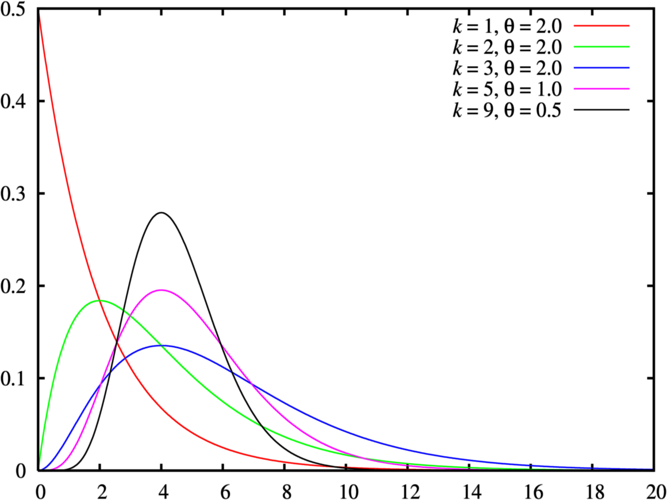
- It turns out that when μ is fixed, a conjugate prior for the precision is the gamma distribution (e.g., Gelman et al., 2013, p. 43).
- It is important to understand the meaning of a gamma prior on precision.
- Consider a gamma distribution
- that is loaded heavily over very small values, but has a long shallow tail extending over large values.
- This sort of gamma distribution on precision indicates that we believe most strongly in small precisions, but we admit that large precisions are possible.
- If this is a belief about the precision of a normal likelihood function, then this sort of gamma distribution expresses a belief that the data will be more spread out, because small precisions imply large standard deviations.
- If the gamma distribution is instead loaded over large values of precision,
- it expresses a belief that the data will be tightly clustered.
- that is loaded heavily over very small values, but has a long shallow tail extending over large values.
참고: gamma distribution ?
conjugate priors & gamma distiribution & precision
- Because of its role in conjugate priors for the normal likelihood function, the gamma distribution is routinely used as a prior on precision.
- But there is no logical necessity to do so, and modern MCMC methods permit more flexible specification of priors.
- Indeed, because precision is less intuitive than standard deviation, it can be more useful instead to give the standard deviation a uniform prior that spans a wide range.
Summary
We have assumed that the data are generated by a normal likelihood function, parameterized by a mean μ and standard deviation σ , and denoted y ∼ normal(y|μ, σ ). For purposes of mathematical derivation, we made unrealistic assumptions that the prior distribution is either a spike on σ or a spike on μ, in order to make three main points:
- A natural way to express a prior on μ is with a normal distribution, because this is conjugate with the normal likelihood when its standard deviation is fixed.
- A way to express a prior on the precision 1/σ 2 is with a gamma distribution, because this is conjugate with the normal likelihood when its mean is fixed. However in practice the standard deviation can instead be given a uniform prior (or anything else that reflects prior beliefs, of course).
- The formulas for Bayesian updating of the parameter distribution are more conveniently expressed in terms of precision than standard deviation. Normal distributions are described sometimes in terms of standard deviation and sometimes in terms of precision, so it is important to glean from context which is being referred to. In R and Stan, the normal distribution is parameterized by mean and standard deviation. In JAGS and BUGS, the normal distribution is parameterized by mean and precision.
16.1.2 Approximation by MCMC in JAGS
It is easy to estimate the mean and standard deviation in JAGS.
- The right panel of Figure 16.2 instead puts a broad uniform distribution directly
on σ . The low and high values of the uniform distribution are set to be far outside any realistic value for the data, so that the prior has minimal influence on the posterior.
- The uniform prior on σ is easier to intuit than a gamma prior on precision, but the priors are not equivalent.

dataList = list(
    y = y ,
    Ntotal = length(y) ,
    meanY = mean(y) ,
    sdY = sd(y)
)
model {
    for ( i in 1:Ntotal ) {
        y[i]  ̃ dnorm( mu , 1/sigmaˆ2 ) # JAGS uses precision
    }
    mu  ̃ dnorm( meanY , 1/(100*sdY)ˆ2 ) # JAGS uses precision
    sigma  ̃ dunif( sdY/1000 , sdY*1000 )
}
- For purposes of illustration, we use fictitious data.
- The data are
- IQ (intelligence quotient) scores
- from a group of people who have consumed a “smart drug.”
- We know that IQ tests have been normed to the general population so that they have an average score of 100 and a standard deviation of 15.
- IQ (intelligence quotient) scores
- Therefore, we would like to know how differently the smart-drug group has performed relative to the general population average.

Jags-Ymet-Xnom1grp-Mnormal-Example.R
# 책에는 없는 코드. 실습을 위해 data 폴더에 넣은 코드를 실행시키기 위한 작업
cur_dir = getwd()
setwd(sprintf("%s/%s", cur_dir, 'data'))
# Example for Jags-Ymet-Xnom1grp-Mnormal.R
#-------------------------------------------------------------------------------
# Optional generic preliminaries:
#graphics.off() # This closes all of R's graphics windows.
#rm(list=ls())  # Careful! This clears all of R's memory!
#-------------------------------------------------------------------------------
# Load The data file
myDataFrame = read.csv( file="TwoGroupIQ.csv" )
myDataFrame
| Score | Group | |
|---|---|---|
| 1 | 102 | Smart Drug |
| 2 | 107 | Smart Drug |
| 3 | 92 | Smart Drug |
| 4 | 101 | Smart Drug |
| 5 | 110 | Smart Drug |
| 6 | 68 | Smart Drug |
| 7 | 119 | Smart Drug |
| 8 | 106 | Smart Drug |
| 9 | 99 | Smart Drug |
| 10 | 103 | Smart Drug |
| 11 | 90 | Smart Drug |
| 12 | 93 | Smart Drug |
| 13 | 79 | Smart Drug |
| 14 | 89 | Smart Drug |
| 15 | 137 | Smart Drug |
| 16 | 119 | Smart Drug |
| 17 | 126 | Smart Drug |
| 18 | 110 | Smart Drug |
| 19 | 71 | Smart Drug |
| 20 | 114 | Smart Drug |
| 21 | 100 | Smart Drug |
| 22 | 95 | Smart Drug |
| 23 | 91 | Smart Drug |
| 24 | 99 | Smart Drug |
| 25 | 97 | Smart Drug |
| 26 | 106 | Smart Drug |
| 27 | 106 | Smart Drug |
| 28 | 129 | Smart Drug |
| 29 | 115 | Smart Drug |
| 30 | 124 | Smart Drug |
| 31 | 137 | Smart Drug |
| 32 | 73 | Smart Drug |
| 33 | 69 | Smart Drug |
| 34 | 95 | Smart Drug |
| 35 | 102 | Smart Drug |
| 36 | 116 | Smart Drug |
| 37 | 111 | Smart Drug |
| 38 | 134 | Smart Drug |
| 39 | 102 | Smart Drug |
| 40 | 110 | Smart Drug |
| 41 | 139 | Smart Drug |
| 42 | 112 | Smart Drug |
| 43 | 122 | Smart Drug |
| 44 | 84 | Smart Drug |
| 45 | 129 | Smart Drug |
| 46 | 112 | Smart Drug |
| 47 | 127 | Smart Drug |
| 48 | 106 | Smart Drug |
| 49 | 113 | Smart Drug |
| 50 | 109 | Smart Drug |
| 51 | 208 | Smart Drug |
| 52 | 114 | Smart Drug |
| 53 | 107 | Smart Drug |
| 54 | 50 | Smart Drug |
| 55 | 169 | Smart Drug |
| 56 | 133 | Smart Drug |
| 57 | 50 | Smart Drug |
| 58 | 97 | Smart Drug |
| 59 | 139 | Smart Drug |
| 60 | 72 | Smart Drug |
| 61 | 100 | Smart Drug |
| 62 | 144 | Smart Drug |
| 63 | 112 | Smart Drug |
| 64 | 109 | Placebo |
| 65 | 98 | Placebo |
| 66 | 106 | Placebo |
| 67 | 101 | Placebo |
| 68 | 100 | Placebo |
| 69 | 111 | Placebo |
| 70 | 117 | Placebo |
| 71 | 104 | Placebo |
| 72 | 106 | Placebo |
| 73 | 89 | Placebo |
| 74 | 84 | Placebo |
| 75 | 88 | Placebo |
| 76 | 94 | Placebo |
| 77 | 78 | Placebo |
| 78 | 108 | Placebo |
| 79 | 102 | Placebo |
| 80 | 95 | Placebo |
| 81 | 99 | Placebo |
| 82 | 90 | Placebo |
| 83 | 116 | Placebo |
| 84 | 97 | Placebo |
| 85 | 107 | Placebo |
| 86 | 102 | Placebo |
| 87 | 91 | Placebo |
| 88 | 94 | Placebo |
| 89 | 95 | Placebo |
| 90 | 86 | Placebo |
| 91 | 108 | Placebo |
| 92 | 115 | Placebo |
| 93 | 108 | Placebo |
| 94 | 88 | Placebo |
| 95 | 102 | Placebo |
| 96 | 102 | Placebo |
| 97 | 120 | Placebo |
| 98 | 112 | Placebo |
| 99 | 100 | Placebo |
| 100 | 105 | Placebo |
| 101 | 105 | Placebo |
| 102 | 88 | Placebo |
| 103 | 82 | Placebo |
| 104 | 111 | Placebo |
| 105 | 96 | Placebo |
| 106 | 92 | Placebo |
| 107 | 109 | Placebo |
| 108 | 91 | Placebo |
| 109 | 92 | Placebo |
| 110 | 123 | Placebo |
| 111 | 61 | Placebo |
| 112 | 59 | Placebo |
| 113 | 105 | Placebo |
| 114 | 184 | Placebo |
| 115 | 82 | Placebo |
| 116 | 138 | Placebo |
| 117 | 99 | Placebo |
| 118 | 93 | Placebo |
| 119 | 93 | Placebo |
| 120 | 72 | Placebo |
summary(myDataFrame)
     Score               Group
 Min.   : 50.00   Placebo   :57
 1st Qu.: 92.75   Smart Drug:63
 Median :102.00
 Mean   :104.13
 3rd Qu.:112.00
 Max.   :208.00
# For purposes of this one-group example, use data from Smart Drug group:
myData = myDataFrame$Score[myDataFrame$Group=="Smart Drug"]
#-------------------------------------------------------------------------------
# Optional: Specify filename root and graphical format for saving output.
# Otherwise specify as NULL or leave saveName and saveType arguments
# out of function calls.
fileNameRoot = "OneGroupIQnormal-"
graphFileType = "png"  #"eps"
#-------------------------------------------------------------------------------
# Load the relevant model into R's working memory:
source("Jags-Ymet-Xnom1grp-Mnormal.R")
*********************************************************************
Kruschke, J. K. (2015). Doing Bayesian Data Analysis, Second Edition:
A Tutorial with R, JAGS, and Stan. Academic Press / Elsevier.
*********************************************************************
Loading required package: coda
#-------------------------------------------------------------------------------
# Generate the MCMC chain:
mcmcCoda = genMCMC( data=myData , numSavedSteps=20000 , saveName=fileNameRoot )
Loading required package: rjags
Linked to JAGS 3.4.0
Loaded modules: basemod,bugs
Compiling model graph
   Resolving undeclared variables
   Allocating nodes
   Graph Size: 79

Initializing model

Burning in the MCMC chain...
Sampling final MCMC chain...
#-------------------------------------------------------------------------------
# Display diagnostics of chain, for specified parameters:
parameterNames = varnames(mcmcCoda) # get all parameter names
for ( parName in parameterNames ) {
  diagMCMC( codaObject=mcmcCoda , parName=parName ,
            saveName=fileNameRoot , saveType=graphFileType )
}
# 창으로 뜨는 것들을 없앤다.
graphics.off()


#-------------------------------------------------------------------------------
# Get summary statistics of chain:
summaryInfo = smryMCMC( mcmcCoda ,
                        compValMu=100.0 , ropeMu=c(99.0,101.0) ,
                        compValSigma=15.0 , ropeSigma=c(14,16) ,
                        compValEff=0.0 , ropeEff=c(-0.1,0.1) ,
                        saveName=fileNameRoot )
show(summaryInfo)
             Mean      Median        Mode     ESS HDImass       HDIlow
mu    107.8278271 107.8114667 107.0894331 20097.3    0.95 101.43788497
sigma  25.9588549  25.7791320  25.0124458 11475.4    0.95  21.46449101
effSz   0.3039062   0.3034737   0.2807922 20000.0    0.95   0.04810492
          HDIhigh CompVal PcntGtCompVal ROPElow ROPEhigh PcntLtROPE PcntInROPE
mu    114.4334683     100         98.95    99.0    101.0       0.41      1.625
sigma  30.6368277      15        100.00    14.0     16.0       0.00      0.000
effSz   0.5540163       0         98.95    -0.1      0.1       0.07      5.650
      PcntGtROPE
mu        97.965
sigma    100.000
effSz     94.280
# Display posterior information:
plotMCMC( mcmcCoda , data=myData ,
          compValMu=100.0 , ropeMu=c(99.0,101.0) ,
          compValSigma=15.0 , ropeSigma=c(14,16) ,
          compValEff=0.0 , ropeEff=c(-0.1,0.1) ,
          pairsPlot=TRUE , showCurve=FALSE ,
          saveName=fileNameRoot , saveType=graphFileType )
graphics.off()


16.2. Outliers and Robust Estimation : The t Distribution
- 16.2.1 Using the t distribution in JAGS
- 16.2.2 Using the t distribution in Stan
When data appear to have outliers
beyond what would be accommodated by a normal distribution, it would be useful to be able to describe the data with a more appropriate distribution that has taller or heavier tails than the normal.
- A well-known distribution with heavy tails is the t distribution[2-6].
- Figure 16.4 shows examples of the t distribution.
- Like the normal distribution, it has two parameters
- that control its mean and its width.
- The standard deviation is controlled indirectly via the t distribution’s “scale” parameter.
- In Figure 16.4, the mean is set to zero and the scale is set to one.
- The t distribution has a third parameter
- that controls the heaviness of its tails,
- which I will refer to as the “normality” parameter,
- ν (Greek letter nu).
- Many people might be familiar with this parameter as the “degrees of freedom” from its use in NHST.
- But because
- we will not be using the t distribution as a sampling distribution,
- and instead we will be using it only as a descriptive shape,
- I prefer to name the parameter by its effect on the distribution’s shape.
- But because
- The normality parameter can range continuously from 1 to ∞. As can be seen in Figure 16.4,
- when ν = 1 the t distribution has very heavy tails, and
- when ν approaches ∞ the t distribution becomes normal.
- that controls the heaviness of its tails,

- Figure 16.5 shows examples of how the t distribution is robust against outliers.
- D = {yi}
- p(D|μ, σ ) <- normal
- p(D|μ, σ , ν) <- t

- It is important to understand that the scale parameter σ in the t distribution is not the standard deviation of the distribution.
- The standard deviation is actually larger than σ because of the heavy tails.
- In fact, when ν drops below 2 (but is still ≥ 1), the standard deviation of the mathematical t distribution goes to infinity.
- For example, in the upper panel of Figure 16.5, ν is only 1.14, which means that the standard deviation of the mathematical t distribution is infinity, even though the sample standard deviation of the data is finite.
- At the same time, the scale parameter of the t distribution has value σ = 1.47.
- For example, in the upper panel of Figure 16.5, ν is only 1.14, which means that the standard deviation of the mathematical t distribution is infinity, even though the sample standard deviation of the data is finite.
- In fact, when ν drops below 2 (but is still ≥ 1), the standard deviation of the mathematical t distribution goes to infinity.
- While this value of the scale parameter is not the standard deviation of the distribution, it does have an intuitive relation to the spread of the data.

- The lower panel of Figure 16.5 uses realistic data that indicates levels of inorganic phosphorous, measured in milligrams per deciliter, in 177 human subjects aged 65 or older.
- The authors of the data (Holcomb & Spalsbury, 2005) intentionally altered a few data points to reflect typical transcription errors and to illustrate methods for detecting and correcting such errors.
- We instead assume that we no longer have access to records of the original individual measurements, and must model the uncorrected data set.
- The t distribution accommodates the outliers and fits the distribution of data much better than the normal.
robust estimation
- The use of a heavy-tailed distribution is often called robust estimation because the estimated value of the central tendency is stable, that is, “robust,” against outliers.
- The t distribution is useful
- as a likelihood function for modeling outliers at the level of observed data. But the t distribution is also useful
- for modeling outliers at higher levels in a hierarchical prior.
16.2.1 Using the t distribution in JAGS
using normal
dataList = list(
    y = y ,
    Ntotal = length(y) ,
    meanY = mean(y) ,
    sdY = sd(y)
)
model {
    for ( i in 1:Ntotal ) {
        y[i]  ̃ dnorm( mu , 1/sigmaˆ2 ) # JAGS uses precision
    }
    mu  ̃ dnorm( meanY , 1/(100*sdY)ˆ2 ) # JAGS uses precision
    sigma  ̃ dunif( sdY/1000 , sdY*1000 )
}
using t
model {
    for ( i in 1:Ntotal ) {
        y[i]  ̃ dt( mu , 1/sigmaˆ2 , nu ) # JAGS: dt uses precision
    }
    mu  ̃ dnorm( meanY , 1/(100*sdY)ˆ2 )
    sigma  ̃ dunif( sdY/1000 , sdY*1000 )
    nu <- nuMinusOne+1       # nu must be >= 1
    nuMinusOne  ̃ dexp(1/29)  # prior on nu-1
}


Jags-Ymet-Xnom1grp-Mrobust-Example.R

# 책에는 없는 코드. 실습을 위해 data 폴더에 넣은 코드를 실행시키기 위한 작업
cur_dir = getwd()
setwd(sprintf("%s/%s", cur_dir, 'data'))
#-------------------------------------------------------------------------------
# Optional generic preliminaries:
graphics.off() # This closes all of R's graphics windows.
rm(list=ls())  # Careful! This clears all of R's memory!
#-------------------------------------------------------------------------------
# Load The data file
myDataFrame = read.csv( file="TwoGroupIQ.csv" )
# For purposes of this one-group example, use data from Smart Drug group:
myData = myDataFrame$Score[myDataFrame$Group=="Smart Drug"]
#-------------------------------------------------------------------------------
# Optional: Specify filename root and graphical format for saving output.
# Otherwise specify as NULL or leave saveName and saveType arguments
# out of function calls.
fileNameRoot = "OneGroupIQrobust-Jags-"
graphFileType = "png" #"eps"
#-------------------------------------------------------------------------------
# Load the relevant model into R's working memory:
source("Jags-Ymet-Xnom1grp-Mrobust.R")
*********************************************************************
Kruschke, J. K. (2015). Doing Bayesian Data Analysis, Second Edition:
A Tutorial with R, JAGS, and Stan. Academic Press / Elsevier.
*********************************************************************
Installing packages into ‘/home/moosung/R/x86_64-pc-linux-gnu-library/3.2’
(as ‘lib’ is unspecified)
Error in contrib.url(repos, type): trying to use CRAN without setting a mirror
#-------------------------------------------------------------------------------
# Generate the MCMC chain:
mcmcCoda = genMCMC( data=myData , numSavedSteps=20000 , saveName=fileNameRoot )
#-------------------------------------------------------------------------------
# Display diagnostics of chain, for specified parameters:
parameterNames = varnames(mcmcCoda) # get all parameter names
for ( parName in parameterNames ) {
  diagMCMC( codaObject=mcmcCoda , parName=parName ,
            saveName=fileNameRoot , saveType=graphFileType )
}
# 창으로 뜨는 것들을 없앤다.
graphics.off()
#-------------------------------------------------------------------------------
# Get summary statistics of chain:
summaryInfo = smryMCMC( mcmcCoda ,
                        compValMu=100.0 , ropeMu=c(99.0,101.0) ,
                        compValSigma=15.0 , ropeSigma=c(14,16) ,
                        compValEff=0.0 , ropeEff=c(-0.1,0.1) ,
                        saveName=fileNameRoot )
show(summaryInfo)
# Display posterior information:
plotMCMC( mcmcCoda , data=myData ,
          compValMu=100.0 , ropeMu=c(99.0,101.0) ,
          compValSigma=15.0 , ropeSigma=c(14,16) ,
          compValEff=0.0 , ropeEff=c(-0.1,0.1) ,
          pairsPlot=TRUE , showCurve=FALSE ,
          saveName=fileNameRoot , saveType=graphFileType )
graphics.off()
16.2.2 Using the t distribution in Stan
- When you run the JAGS program yourself, you will see that it uses many steps to produce a posterior sample for σ that has an ESS exceeding 10,000.
- You will also see that the ESS for ν is less than 10,000 despite the long chain.
- In other words, there is high autocorrelation in the chains in JAGS.
- We do not care that the chain for ν has a relatively small ESS because
- (a) we do not care about the exact value of ν when interpreting the posterior, as explained above, and
- (b) the exact value of ν has relatively little effect on the estimates of the other parameters.
- To be sure, the posterior sample of ν must be converged and truly representative of the posterior, but it does not need to be as finely detailed as the other parameters.
- Nevertheless, it would be less worrying if ν had a larger ESS.
- The autocorrelation of the MCMC sampling in JAGS requires a long chain,
- which requires us to have patience while the computer chugs along.
- We have discussed two options for improving the efficiency of the sampling.
- One option is to run parallel chains on multiple cores using runjags (Section 8.7, p. 215).
- Another option is to implement the model in Stan,
- which may explore the parameter space more efficiently with its HMC sampling (Chapter 14).
- The autocorrelation of the MCMC sampling in JAGS requires a long chain,
- This section shows how to run the model in Stan. Its results do indeed show a posterior sample of ν with higher ESS than JAGS.
data {
    int<lower=1> Ntotal ;
    real y[Ntotal] ;
    real meanY ;
    real sdY ;
}
transformed data { // compute the constants for the priors
    real unifLo ;
    real unifHi ;
    real normalSigma ;
    real expLambda ;
    unifLo <- sdY/1000 ;
    unifHi <- sdY*1000 ;
    normalSigma <- sdY*100 ;
    expLambda <- 1/29.0 ;
}
parameters {
    real<lower=0> nuMinusOne ;
    real mu ;
    real<lower=0> sigma ;
}
transformed parameters {
    real<lower=0> nu ;
    nu <- nuMinusOne + 1 ;
}
model {
    sigma  ̃ uniform( unifLo , unifHi ) ;
    mu  ̃ normal( meanY , normalSigma ) ;
    nuMinusOne  ̃ exponential( expLambda ) ;
    y  ̃ student_t( nu , mu , sigma ) ; // vectorized
}


Stan-Ymet-Xnom1grp-Mrobust-Example.R
# 책에는 없는 코드. 실습을 위해 data 폴더에 넣은 코드를 실행시키기 위한 작업
cur_dir = getwd()
setwd(sprintf("%s/%s", cur_dir, 'data'))
#-------------------------------------------------------------------------------
# Optional generic preliminaries:
graphics.off() # This closes all of R's graphics windows.
rm(list=ls())  # Careful! This clears all of R's memory!
#-------------------------------------------------------------------------------
# Load The data file
myDataFrame = read.csv( file="TwoGroupIQ.csv" )
# For purposes of this one-group example, use data from Smart Drug group:
myData = myDataFrame$Score[myDataFrame$Group=="Smart Drug"]
#-------------------------------------------------------------------------------
# Load the relevant model into R's working memory:
source("Stan-Ymet-Xnom1grp-Mrobust.R")
#-------------------------------------------------------------------------------
# Optional: Specify filename root and graphical format for saving output.
# Otherwise specify as NULL or leave saveName and saveType arguments
# out of function calls.
fileNameRoot = "OneGroupIQrobust-Stan-"
graphFileType = "png" #"eps"
#-------------------------------------------------------------------------------
# Generate the MCMC chain:
mcmcCoda = genMCMC( data=myData , numSavedSteps=20000 , saveName=fileNameRoot )
#-------------------------------------------------------------------------------
# Display diagnostics of chain, for specified parameters:
parameterNames = varnames(mcmcCoda) # get all parameter names
for ( parName in parameterNames ) {
  diagMCMC( codaObject=mcmcCoda , parName=parName ,
            saveName=fileNameRoot , saveType=graphFileType )
}
# 창으로 뜨는 것들을 없앤다.
graphics.off()
#-------------------------------------------------------------------------------
# Get summary statistics of chain:
summaryInfo = smryMCMC( mcmcCoda ,
                        compValMu=100.0 , ropeMu=c(99.0,101.0) ,
                        compValSigma=15.0 , ropeSigma=c(14,16) ,
                        compValEff=0.0 , ropeEff=c(-0.1,0.1) ,
                        saveName=fileNameRoot )
show(summaryInfo)
# Display posterior information:
plotMCMC( mcmcCoda , data=myData ,
          compValMu=100.0 , ropeMu=c(99.0,101.0) ,
          compValSigma=15.0 , ropeSigma=c(14,16) ,
          compValEff=0.0 , ropeEff=c(-0.1,0.1) ,
          pairsPlot=TRUE , showCurve=FALSE ,
          saveName=fileNameRoot , saveType=graphFileType )
graphics.off()
16.3. Two Groups
- 16.3.1 Analysis by NHST
An often-used research design is a comparison of two groups.
- For example, in the context of assaying the effect of a “smart drug” on IQ, instead of comparing the mean of the treatment group against an assumed landmark such as 100 (see Figure 16.3), it would make more sense to compare the treatment group against an identically handled placebo group.
- When there are two groups, we estimate the mean and scale for each group.
- When using t distributions for robust estimation,
- we could also estimate the normality of each group separately.
- But because there usually are relatively few outliers,
- we will use a single normality parameter to describe both groups,
- so that the estimate of the normality is more stably estimated.
- we will use a single normality parameter to describe both groups,

data {
    int<lower=1> Ntotal ;
    int x[Ntotal] ;                                                 // group identifier
    real y[Ntotal] ;
    real meanY ;
    real sdY ;
}
transformed data {
    real unifLo ;
    real unifHi ;
    real normalSigma ;
    real expLambda ;
    unifLo <- sdY/1000 ;
    unifHi <- sdY*1000 ;
    normalSigma <- sdY*100 ;
    expLambda <- 1/29.0 ;
}
parameters {
    real<lower=0> nuMinusOne ;
    real mu[2] ;                                                   // 2 groups
    real<lower=0> sigma[2] ;                               // 2 groups
}
transformed parameters {
    real<lower=0> nu ;
    nu <- nuMinusOne + 1 ;
}
model {
    sigma  ̃ uniform( unifLo , unifHi ) ;                    // vectorized 2 groups
    mu  ̃ normal( meanY , normalSigma ) ;             // vectorized 2 groups
    nuMinusOne  ̃ exponential( expLambda ) ;
    for ( i in 1:Ntotal ) {
        y[i]  ̃ student_t( nu , mu[x[i]] , sigma[x[i]] ) ;
    }
}

Stan-Ymet-Xnom1grp-Mrobust-Example.R
#-------------------------------------------------------------------------------
# Optional generic preliminaries:
graphics.off() # This closes all of R's graphics windows.
rm(list=ls())  # Careful! This clears all of R's memory!
#-------------------------------------------------------------------------------
# Load The data file
myDataFrame = read.csv( file="TwoGroupIQ.csv" )
# For purposes of this one-group example, use data from Smart Drug group:
myData = myDataFrame$Score[myDataFrame$Group=="Smart Drug"]
#-------------------------------------------------------------------------------
# Load the relevant model into R's working memory:
source("Stan-Ymet-Xnom1grp-Mrobust.R")
#-------------------------------------------------------------------------------
# Optional: Specify filename root and graphical format for saving output.
# Otherwise specify as NULL or leave saveName and saveType arguments
# out of function calls.
fileNameRoot = "OneGroupIQrobust-Stan-"
graphFileType = "png" #"eps"
#-------------------------------------------------------------------------------
# Generate the MCMC chain:
mcmcCoda = genMCMC( data=myData , numSavedSteps=20000 , saveName=fileNameRoot )
#-------------------------------------------------------------------------------
# Display diagnostics of chain, for specified parameters:
parameterNames = varnames(mcmcCoda) # get all parameter names
for ( parName in parameterNames ) {
  diagMCMC( codaObject=mcmcCoda , parName=parName ,
            saveName=fileNameRoot , saveType=graphFileType )
}
# 창으로 뜨는 것들을 없앤다.
graphics.off()
#-------------------------------------------------------------------------------
# Get summary statistics of chain:
summaryInfo = smryMCMC( mcmcCoda ,
                        compValMu=100.0 , ropeMu=c(99.0,101.0) ,
                        compValSigma=15.0 , ropeSigma=c(14,16) ,
                        compValEff=0.0 , ropeEff=c(-0.1,0.1) ,
                        saveName=fileNameRoot )
show(summaryInfo)
graphics.off()
# Display posterior information:
plotMCMC( mcmcCoda , data=myData ,
          compValMu=100.0 , ropeMu=c(99.0,101.0) ,
          compValSigma=15.0 , ropeSigma=c(14,16) ,
          compValEff=0.0 , ropeEff=c(-0.1,0.1) ,
          pairsPlot=TRUE , showCurve=FALSE ,
          saveName=fileNameRoot , saveType=graphFileType )
graphics.off()
16.3.1 Analysis by NHST
- In traditional NHST, metric data from two groups would be submitted to a t-test.
myDataFrame = read.csv( file="TwoGroupIQ.csv" )
t.test(Score~Group , data=myDataFrame)
	Welch Two Sample t-test

data:  Score by Group
t = -1.958, df = 111.44, p-value = 0.05273
alternative hypothesis: true difference in means is not equal to 0
95 percent confidence interval:
 -15.70602585   0.09366161
sample estimates:
   mean in group Placebo mean in group Smart Drug
                100.0351                 107.8413
- Notice that the p value is greater than 0.05, which means that the conventional decision would be not to reject the null hypothesis.
- This conclusion conflicts with the Bayesian analysis in Figure 16.12, unless we use a conservatively wide ROPE.
- The reason that
- the t test is less sensitive than the Bayesian estimation
- in this example is that
- the t test assumes normality and therefore
- its estimate of the within-group variances is too large
- when there are outliers.
- in this example is that
- the t test is less sensitive than the Bayesian estimation
- The t test has other problems. Unlike the Bayesian analysis,
- the t test provides only a test of the equality of means,
- without a test of the equality of variances.
- To test equality of variances,
- we need to run an additional test,
- namely an F test of the ratio of variances, which would inflate the p values of both tests.
- we need to run an additional test,
- Moreover,
- both tests compute p values based on hypothetical normally distributed data,
- and the F test is particularly sensitive to violations of this assumption.
- the t test provides only a test of the equality of means,
- Therefore it would be better to use resampling methods to compute the p values (and correcting them for multiple tests).
16.4. Other Noise Distributions and Transforming Data
16.5. EXERCISES
Exercise 16.1.
[Purpose: Practice using different data files in the high-level script, with an interesting real example about alcohol preference of sexually frustrated males.]

참고자료
- [1] Doing Bayesian Data Analysis, Second Edition: A Tutorial with R, JAGS, and Stan - http://www.amazon.com/Doing-Bayesian-Analysis-Second-Edition/dp/0124058884
- [2] 스튜던트 t 분포(한글위키피디아) - https://ko.wikipedia.org/wiki/%EC%8A%A4%ED%8A%9C%EB%8D%98%ED%8A%B8_t_%EB%B6%84%ED%8F%AC
- [3] t분포(티분포) 개념정리! - http://math7.tistory.com/55
- [4] t분포표(티분포표) 보는 법! - http://math7.tistory.com/56
- [5] 표준정규분포와 t분포의 차이 - http://blog.daum.net/_blog/BlogTypeView.do?blogid=0Isuz&articleno=1172552
- [6] t 분포 (Student's t-distribution) - http://godrag77.blogspot.kr/2011/07/t-students-t-distribution.html