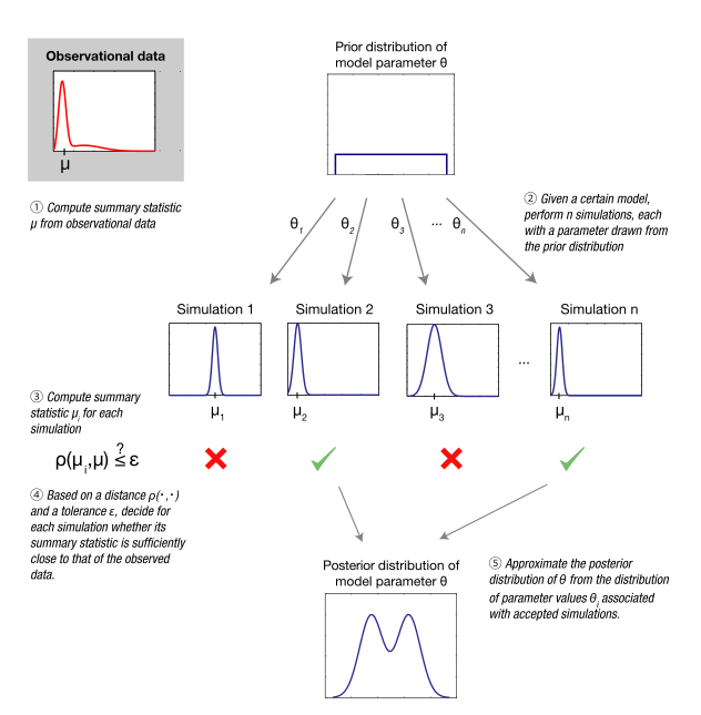
Chapter 10 Approximate Bayesian Computation
(이하 abc 방법)
10.1 변이 가설(The Variability Hypothesis)
다루려고 하는 내용: 변이가설
조안미켈의 믿음: 대부분의 천재와 대부분의 정식적 미숙아는 남자다 그는 남자는 우수한 동물이라고 생각해서 여성의 변이 부족은 열등함의 표시라고 결론지었다. 최근 수업에서 CDC의 행동 위험 요인 감시 시스템에서 미국의 남(15,507명)녀(254,722명) 성인이 키를 직접 입력한 데이터의 결과는 다음과 같다.
남성의 평균 키는 178cm이고 여성의 평균 키는 163cm이다. 즉 평균적으로 남성의 키가 더 가변적이다. 남성의 표준편차는 7.7cm이고 여성의 경우는 7.3cm다. 따라서 절대적으로 남성의 키다 더 가변적이다. 하지만 그룹간의 변이를 비교할 때 표준편차를 평균으로 나눈 변동 계수coefficient of variation (CV)를 사용하면 더 의미가 있다. 이 값은 변이가 원 수치와 관계없는 무차원적 측정치다. 남성의 경우 CV가 0.044333이고 여성의 경우 0.0444이다. 숫자들이 비슷하여 변이가설을 증명하기에는 빈약하다고 결론 내릴 수 있다. 하지만 베이지안 매서드를 사용하여 결론을 더 명확하게 만들 수 있다.
큰 데이터셋을 다루는 몇 가지 기술
- 우선 간단한 구현 내용에서 시작한다. 하지만 이 구현 내용은 1.000개 이하의 데이터셋에서만 동작한다.
- 로그 변환하려면 확률을 계산하려면 전체 데이터셋을 스케일 변환을 해야 하지만 그럼 계산 속도가 느려진다.
- 마지막으로 보통 ABC로 알려져 있는 근사 베이지안 계산을 통해 속도를 꽤 높일 것이다.
import math
import numpy
import cPickle
import random
import scipy

import brfss

import thinkplot
import thinkbayes
import thinkstats

import matplotlib.pyplot as pyplot


NUM_SIGMAS = 1
10.2 평균과 표준편차
이 장에서는 가우시안 분표의 변수인 평균 mu(mean)와 표준편차sigma(the standard deviation)를 동일한 방식으로 추정할 것이다. 그리고 이 문제에서는 의 mu와 sigma의 쌍과 이 쌍이 나타날 확률의 연결 내용을 만드는 Height라고 부르는 Suite 를 정의하겠다.
8장 잠깐 복습) 스윗(Suite): 가설집합
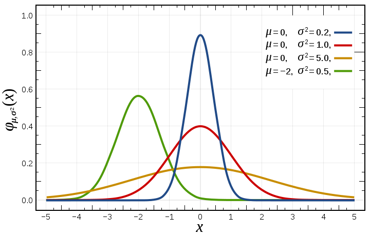
Normalized Gaussian curves with expected value μ and variance σ2. The corresponding parameters are a = \tfrac{1}{\sigma\sqrt{2\pi}}, b = μ, and c = σ.
mus는 mu의 가능한 값의 연속이고 sigmas는 sigma의 값의 연속이다. 모든 mu, sigma 쌍의 사전 분포는 균등 분포다. 이에 대한 우도 함수는 쉽다. mu, sigma의 가설 값이 주어졌을 때 특정 값 x에 대한 우도를 계산할 수 있다. 이 기능은 EvalGaussianpdf가 수행하므로 우리는 이 함수를 실행하기만 하면 된다.
이 문제의 가장 어려운 부분은 mus 와 sigma를 구하는 것이다. 따라서 베이지안 기술을 더 효율적으로 쓰기 위해 고전적 추정치를 사용하고 이 추정값의 적절한 분포를 선택하기 위해 표준편차를 사용하려 한다. 분포의 진짜 변수가 µ 와 σ 이고 여기서 n개의 샘플을 취했을 때 µ의 추정치는 샘플 평균인 m이다. 또한 σ 의 추정치는 샘플 표준편차인 s다. 추청된 µ 의 표준편차는 s / √n 이고 σ의 추정치의 s / √2 (n−1)이다.
10.3 갱신(Update)
이 프로세스는 허위 같다. 우리는 사전 분포에서 데이터의 범위를 선택한 수 갱신한 데이터를 다시 사용한다. 보통 같은 데이터를 두 번 사용하면 사실 허위다. 하지만 이 경우에는 괜찮다. 사실이다. 우리는 사전 분포의 범위에서 데이터를 선택한 이유는 수많은 매우 작은 값에 대해서는 계산하지 않기 위해서일 뿐이다. 실제로는 사전 분포는 mus와 sigma의 모든 값에 대해 균등 분포지만, 계산 효율성을 위해 필요 없는 값들을 모두 무시하다.
10.4 CV의 사후 분포
한 번 mu와 sigma의 사후 결합 분포를 계산해 놓으면 남녀의 CV의 분포와 한 쪽이 다른 쪽을 넘어설 확률을 계산할 수 있다. CV의 분포 계산을 위해 mu와 sigma의 쌍을 만들 것이다.
10.5 언더플로
(소수점 이하 연산 제한의 문제를 해결하기 위한 과정) 그 후 thinkbayes.PmfProbGreater를 사용해서 남자가 더 변이 성이 높을 확률을 계산할 것이다. 우도 계산에 확률 밀도를 사용하는데 연속형 분포의 경우 밀도가 매우 작아서 0으로 수렴하는데 이를 해결하기 위해 로그 변환하에 우도를 계산한다.
log는 pmf내의 확률 로그를 계산한다.
class Height(thinkbayes.Suite, thinkbayes.Joint):
    """Hypotheses about parameters of the distribution of height."""

    def __init__(self, mus, sigmas, name=''):
        """Makes a prior distribution for mu and sigma based on a sample.

        mus: sequence of possible mus
        sigmas: sequence of possible sigmas
        name: string name for the Suite
        """
        pairs = [(mu, sigma)
                 for mu in mus
                 for sigma in sigmas]

        thinkbayes.Suite.__init__(self, pairs, name=name)

    def Likelihood(self, data, hypo):
        """Computes the likelihood of the data under the hypothesis.

        Args:
            hypo: tuple of hypothetical mu and sigma
            data: float sample

        Returns:
            likelihood of the sample given mu and sigma
        """
        x = data
        mu, sigma = hypo
        like = scipy.stats.norm.pdf(x, mu, sigma)
        return like

    def LogLikelihood(self, data, hypo):
        """Computes the log likelihood of the data under the hypothesis.

        Args:
            data: a list of values
            hypo: tuple of hypothetical mu and sigma

        Returns:
            log likelihood of the sample given mu and sigma (unnormalized)
        """
        x = data
        mu, sigma = hypo
        loglike = EvalGaussianLogPdf(x, mu, sigma)
        return loglike

    def LogUpdateSetFast(self, data):
        """Updates the suite using a faster implementation.

        Computes the sum of the log likelihoods directly.

        Args:
            data: sequence of values
        """
        xs = tuple(data)
        n = len(xs)

        for hypo in self.Values():
            mu, sigma = hypo
            total = Summation(xs, mu)
            loglike = -n * math.log(sigma) - total / 2 / sigma**2
            self.Incr(hypo, loglike)

    def LogUpdateSetMeanVar(self, data):
        """Updates the suite using ABC and mean/var.

        Args:
            data: sequence of values
        """
        xs = data
        n = len(xs)

        m = numpy.mean(xs)
        s = numpy.std(xs)

        self.LogUpdateSetABC(n, m, s)

    def LogUpdateSetMedianIPR(self, data):
        """Updates the suite using ABC and median/iqr.

        Args:
            data: sequence of values
        """
        xs = data
        n = len(xs)

        # compute summary stats
        median, s = MedianS(xs, num_sigmas=NUM_SIGMAS)
        print 'median, s', median, s

        self.LogUpdateSetABC(n, median, s)

    def LogUpdateSetABC(self, n, m, s):
        """Updates the suite using ABC.

        n: sample size
        m: estimated central tendency
        s: estimated spread
        """
        for hypo in sorted(self.Values()):
            mu, sigma = hypo

            # compute log likelihood of m, given hypo
            stderr_m = sigma / math.sqrt(n)
            loglike = EvalGaussianLogPdf(m, mu, stderr_m)

            #compute log likelihood of s, given hypo
            stderr_s = sigma / math.sqrt(2 * (n-1))
            loglike += EvalGaussianLogPdf(s, sigma, stderr_s)

            self.Incr(hypo, loglike)
10.6 로그 우도
이제 우리가 필요한 것은 likelihood뿐이다. logPdf는 가우시안 PDF의 로그 우도를 계산하고 갱신한다.
10.7 약간의 최적화
LogUpdateSet을 각 데이터 지점에 대해 한 번씩 LogUpdate를 호출한다. 이를 전체 데이터셋에 대해 우도를 한 번에 계산하면 개선할 수 있다.
10.8 근사베이지안 계산(ABC)
ABC는 어떤 특정 데이터셋의 우도가 다음과 같을 때 사용한다.
- 특히 큰 데이텃셋의 경우, 매우 작아서 로그 변환이 어려운 경우
- 계산 비용이 많이 들어서 최적화를 많이 해야 하는 경우
- 어쨌든 별로 하기 싫은 경우
우리는 우리가 본 정확한 데이터셋을 보는 것에 대한 우도가 어떻든 별로 상관없다. 특히 연속형변수의 경우 우리가 본 것과 같은 모든 데이터셋을 보게 되는 것에 대한 우도에만 신경쓴다. 그리고 결국 가우시안 분포에서 샘플링을 하면 이미 샘플 통계에서 분포를 정확히 찾아낼 수 잇기 때문에 보다 표과적으로 답을 찾아낼 수 있다. 사실 이미 사전 범위를 계산하면서 이에 대한 내용을 했었다. 우리는 이 샘플 분포를 사용해서 µ와 σ 의 가설 값이 주어졌을 때 샘플 통계의 우도를 계산할 수 있다.
보충)근사 베이지안과 pure베이지안의 가장 큰 차이는 뭐가 있을까요? 답: Exact Bayesian Inference는 사후분포를 정확하게 알아내기 위한 기법인데 대표적인 것은 MCMC입니다. 대개 Exact Bayes 기법들은 정확하지만 계산적 비용이 많이 듭니다. 이것을 해결하기 위해 나온 게 Approximate computation 기법들인데, 이 기법들의 목적은 사후분포를 정확하게 알아내는 것이 아니라 대충, 그러나 될 수 있는 한 최대한 가깝게 근사하는 것입니다. (당연히 계산시간이 단축되겠죠) 몇 가지 기법들이 있는데, variational Bayes (VB) 는 임의의 분포족에서 원래 분포에 가장 가깝게 근사할 수 있는 분포를 찾는 게 목적이고, MCMC에 비해 계산시간이 상당히 단축됩니다. INLA 라는 기법도 있는데, 정규분포 근사 기법이라고 알고 있는데 확실한지는 모르겠습니다. 마지막으로 최근에는 ABC (approximate Bayesian computation) 이라고 해서 별도의 기법도 나왔는데, 이 기법은 likelihood-free 라고 해서 사후분포의 식 자체가 필요없는 신기한 기법입니다.
def EvalGaussianLogPdf(x, mu, sigma):
    """Computes the log PDF of x given mu and sigma.

    x: float values
    mu, sigma: paramemters of Gaussian

    returns: float log-likelihood
    """
    return scipy.stats.norm.logpdf(x, mu, sigma)


def FindPriorRanges(xs, num_points, num_stderrs=3.0, median_flag=False):
    """Find ranges for mu and sigma with non-negligible likelihood.

    xs: sample
    num_points: number of values in each dimension
    num_stderrs: number of standard errors to include on either side

    Returns: sequence of mus, sequence of sigmas
    """
    def MakeRange(estimate, stderr):
        """Makes a linear range around the estimate.

        estimate: central value
        stderr: standard error of the estimate

        returns: numpy array of float
        """
        spread = stderr * num_stderrs
        array = numpy.linspace(estimate-spread, estimate+spread, num_points)
        #* numpy.linspace는 estimate-spread와 estimate+spread 사이에 이 두 값을 포함하여 간격이 동일한 원소들의 행렬이다.
        return array

    # estimate mean and stddev of xs
    n = len(xs)
    if median_flag:
        m, s = MedianS(xs, num_sigmas=NUM_SIGMAS)
    else:
        m = numpy.mean(xs)
        s = numpy.std(xs)

    print 'classical estimators', m, s

    # compute ranges for m and s
    stderr_m = s / math.sqrt(n)
    mus = MakeRange(m, stderr_m)

    stderr_s = s / math.sqrt(2 * (n-1))
    sigmas = MakeRange(s, stderr_s)

    return mus, sigmas
10.9 로버스트 추정
229cm인 여성 4명이 극단값일 확률이 있다. 이럴 때는 분포 p의 주어진 어느 범위 내의 차잇값을 구하는 분위 내 범위interpercentile range.IPR를 계산할 수 있다.  이 때 p=0.5는 4분위 범위가 된다.

다시 한 번 확인하자. xs는 값의 연속값이고 num_sigmas는 기반이 되는 결과의 표준편차 숫자다. 결과는 µ 를 추정하는 median과 σ를 추정하는 s다. 마지막으로 LofUpdataSetABC에서 샘플 평균과 표준편차를 median과 S로 치환할 수 있다. 다른 것도 비슷하다.
def CoefVariation(suite):
    """Computes the distribution of CV.

    suite: Pmf that maps (x, y) to z

    Returns: Pmf object for CV.
    """
    pmf = thinkbayes.Pmf()
    for (m, s), p in suite.Items():
        pmf.Incr(s/m, p)
    return pmf


def PlotCdfs(d, labels):
    """Plot CDFs for each sequence in a dictionary.

    Jitters the data and subtracts away the mean.

    d: map from key to sequence of values
    labels: map from key to string label
    """
    thinkplot.Clf()
    for key, xs in d.iteritems():
        mu = thinkstats.Mean(xs)
        xs = thinkstats.Jitter(xs, 1.3)
        xs = [x-mu for x in xs]
        cdf = thinkbayes.MakeCdfFromList(xs)
        thinkplot.Cdf(cdf, label=labels[key])
    thinkplot.Show()


def PlotPosterior(suite, pcolor=False, contour=True):
    """Makes a contour plot.

    suite: Suite that maps (mu, sigma) to probability
    """
    thinkplot.Clf()
    thinkplot.Contour(suite.GetDict(), pcolor=pcolor, contour=contour)

    thinkplot.Save(root='variability_posterior_%s' % suite.name,
                title='Posterior joint distribution',
                xlabel='Mean height (cm)',
                ylabel='Stddev (cm)')


def PlotCoefVariation(suites):
    """Plot the posterior distributions for CV.

    suites: map from label to Pmf of CVs.
    """
    thinkplot.Clf()
    thinkplot.PrePlot(num=2)

    pmfs = {}
    for label, suite in suites.iteritems():
        pmf = CoefVariation(suite)
        print 'CV posterior mean', pmf.Mean()
        cdf = thinkbayes.MakeCdfFromPmf(pmf, label)
        thinkplot.Cdf(cdf)

        pmfs[label] = pmf

    thinkplot.Save(root='variability_cv',
                xlabel='Coefficient of variation',
                ylabel='Probability')

    print 'female bigger', thinkbayes.PmfProbGreater(pmfs['female'],
                                                     pmfs['male'])
    print 'male bigger', thinkbayes.PmfProbGreater(pmfs['male'],
                                                   pmfs['female'])


def PlotOutliers(samples):
    """Make CDFs showing the distribution of outliers."""
    cdfs = []
    for label, sample in samples.iteritems():
        outliers = [x for x in sample if x < 150]

        cdf = thinkbayes.MakeCdfFromList(outliers, label)
        cdfs.append(cdf)

    thinkplot.Clf()
    thinkplot.Cdfs(cdfs)
    thinkplot.Save(root='variability_cdfs',
                title='CDF of height',
                xlabel='Reported height (cm)',
                ylabel='CDF')


def PlotMarginals(suite):
    """Plots marginal distributions from a joint distribution.

    suite: joint distribution of mu and sigma.
    """
    thinkplot.Clf()

    pyplot.subplot(1, 2, 1)
    pmf_m = suite.Marginal(0)
    cdf_m = thinkbayes.MakeCdfFromPmf(pmf_m)
    thinkplot.Cdf(cdf_m)

    pyplot.subplot(1, 2, 2)
    pmf_s = suite.Marginal(1)
    cdf_s = thinkbayes.MakeCdfFromPmf(pmf_s)
    thinkplot.Cdf(cdf_s)

    thinkplot.Show()


def DumpHeights(data_dir='.', n=10000):
    """Read the BRFSS dataset, extract the heights and pickle them."""
    resp = brfss.Respondents()
    resp.ReadRecords(data_dir, n)

    d = {1:[], 2:[]}
    [d[r.sex].append(r.htm3) for r in resp.records if r.htm3 != 'NA']

    fp = open('variability_data.pkl', 'wb')
    cPickle.dump(d, fp)
    fp.close()


def LoadHeights():
    """Read the pickled height data.

    returns: map from sex code to list of heights.
    """
    fp = open('variability_data.pkl', 'r')
    d = cPickle.load(fp)
    fp.close()
    return d


def UpdateSuite1(suite, xs):
    """Computes the posterior distibution of mu and sigma.

    Computes untransformed likelihoods.

    suite: Suite that maps from (mu, sigma) to prob
    xs: sequence
    """
    suite.UpdateSet(xs)


def UpdateSuite2(suite, xs):
    """Computes the posterior distibution of mu and sigma.

    Computes log likelihoods.

    suite: Suite that maps from (mu, sigma) to prob
    xs: sequence
    """
    suite.Log()
    suite.LogUpdateSet(xs)
    suite.Exp()
    suite.Normalize()


def UpdateSuite3(suite, xs):
    """Computes the posterior distibution of mu and sigma.

    Computes log likelihoods efficiently.

    suite: Suite that maps from (mu, sigma) to prob
    t: sequence
    """
    suite.Log()
    suite.LogUpdateSetFast(xs)
    suite.Exp()
    suite.Normalize()


def UpdateSuite4(suite, xs):
    """Computes the posterior distibution of mu and sigma.

    Computes log likelihoods efficiently.

    suite: Suite that maps from (mu, sigma) to prob
    t: sequence
    """
    suite.Log()
    suite.LogUpdateSetMeanVar(xs)
    suite.Exp()
    suite.Normalize()


def UpdateSuite5(suite, xs):
    """Computes the posterior distibution of mu and sigma.

    Computes log likelihoods efficiently.

    suite: Suite that maps from (mu, sigma) to prob
    t: sequence
    """
    suite.Log()
    suite.LogUpdateSetMedianIPR(xs)
    suite.Exp()
    suite.Normalize()


def MedianIPR(xs, p):
    """Computes the median and interpercentile range.

    xs: sequence of values
    p: range (0-1), 0.5 yields the interquartile range

    returns: tuple of float (median, IPR)
    """
    cdf = thinkbayes.MakeCdfFromList(xs)
    median = cdf.Percentile(50)

    alpha = (1-p) / 2
    ipr = cdf.Value(1-alpha) - cdf.Value(alpha)
    return median, ipr


def MedianS(xs, num_sigmas):
    """Computes the median and an estimate of sigma.

    Based on an interpercentile range (IPR).

    factor: number of standard deviations spanned by the IPR
    """
    half_p = thinkbayes.StandardGaussianCdf(num_sigmas) - 0.5
    median, ipr = MedianIPR(xs, half_p * 2)
    s = ipr / 2 / num_sigmas

    return median, s

def Summarize(xs):
    """Prints summary statistics from a sequence of values.

    xs: sequence of values
    """
    # print smallest and largest
    xs.sort()
    print 'smallest', xs[:10]
    print 'largest', xs[-10:]

    # print median and interquartile range
    cdf = thinkbayes.MakeCdfFromList(xs)
    print cdf.Percentile(25), cdf.Percentile(50), cdf.Percentile(75)


def RunEstimate(update_func, num_points=31, median_flag=False):
    """Runs the whole analysis.

    update_func: which of the update functions to use
    num_points: number of points in the Suite (in each dimension)
    """
    # DumpHeights(n=10000000)
    d = LoadHeights()
    labels = {1:'male', 2:'female'}

    # PlotCdfs(d, labels)

    suites = {}
    for key, xs in d.iteritems():
        name = labels[key]
        print name, len(xs)
        Summarize(xs)

        xs = thinkstats.Jitter(xs, 1.3)

        mus, sigmas = FindPriorRanges(xs, num_points, median_flag=median_flag)
        suite = Height(mus, sigmas, name)
        suites[name] = suite
        update_func(suite, xs)
        print 'MLE', suite.MaximumLikelihood()

        PlotPosterior(suite)

        pmf_m = suite.Marginal(0)
        pmf_s = suite.Marginal(1)
        print 'marginal mu', pmf_m.Mean(), pmf_m.Var()
        print 'marginal sigma', pmf_s.Mean(), pmf_s.Var()

        # PlotMarginals(suite)

    PlotCoefVariation(suites)


def main():
    random.seed(17)

    func = UpdateSuite5
    median_flag = (func == UpdateSuite5)
    RunEstimate(func, median_flag=median_flag)


if __name__ == '__main__':
    main()
male 154407
smallest [61, 74, 76, 81, 86, 89, 89, 91, 97, 101]
largest [218, 221, 221, 221, 221, 225, 226, 229, 229, 236]
173 178 183
classical estimators 178.502463829 7.3174757232
median, s 178.502463829 7.3174757232
MLE (178.50246382866365, 7.3174757232006442)
Writing variability_posterior_male.pdf
Writing variability_posterior_male.eps
marginal mu 178.502463829 0.000339825096128
marginal sigma 7.31751710032 0.000169913050402
female 254722
smallest [61, 61, 64, 66, 74, 81, 89, 89, 89, 91]
largest [213, 213, 213, 213, 221, 226, 229, 229, 229, 229]
157 163 168
classical estimators 163.492172625 7.01169223128
median, s 163.492172625 7.01169223128
MLE (163.49217262460459, 7.0116922312800511)
Writing variability_posterior_female.pdf
Writing variability_posterior_female.eps
marginal mu 163.492172625 0.000189137323477
marginal sigma 7.01171626522 9.45688312182e-05
CV posterior mean 0.0409939281588
CV posterior mean 0.0428871682495
Writing variability_cv.pdf
Writing variability_cv.eps
female bigger 1.0
male bigger 0.0
10.10 누가 더 변이성이 높은가
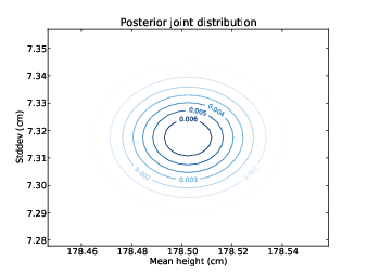
num_sigmas = 1 일 ㄸ 중간값과 IPR기반의 ABC를 사용해서 mu와 sigma 기반의 사후 결합 분표를 계산한다. 그럼 10-1과 10-2는 결과에 대해 x측으로 mu를 넣고 y축으로 sigma를 놓고, z축에 확률을 놓은 등고선 그래프를 보여준다.
그림 10 -1 미국 남성의 키의 평균과 표준편차에 대한 사후 결합 분포의 등고선
각 결합 분포에 대해 CV의 사후 분포를 계산하였다. 그림 10-3은 남녀에 대한 이런 분포를 보여준다. 남성이 평균은 0.041, 여성 평균은 0.0429다. 이 분포 간에 겹치는 부분이 없으므로 여성이 키에 있어서는 남성보다 변이성이 더 높다는 결론을 더 확실하게 낼 수 있다.
그림10-2 미국 여성의 키의 평균고 표준편차에 대한 사후 결합 분포의 등고선

그럼 이제 변이 가설은 끝인가? 아직 아니다. 이 결과는 분위 내 범위 선택에 따라 달라진다는 것으로 밝혀졌다. num_sigmas=2 인 경우 남성이 더 변이성이 높다는 가설이 동일한 신뢰도를 가진다. 이런 차이가 발생하는 원인은 작은 쪽에 치우친 경우가 남성이 더 많고 따라서 평균으로부터의 거리도 커진다. 따라서 변이 가설 평가는 변이(variability)해석에 따라 달라진다. num_sigmas=1일 때 사람들이 평균 부근에 많다는 것에 집중하자. num_sigmas가 증가할수록 극단값의 비중이 높아진다. 결론: 아직은 모호함
그림 10-3 로버스트 추정에 의한 남성과 여성의 CV의 사후 분포

참고자료: 앨런B다우니,(2014) 파이썬을 이용한 베이지안 통계, 한빛미디어 저자 블로그: http://allendowney.blogspot.kr/ 코드: https://github.com/AllenDowney/ThinkBayes 책:http://www.greenteapress.com/thinkbayes/ 고전적 추정치: http://www.amstat.org/publications/jse/v6n3/rossman.html http://www.amstat.org/publications/jse/v9n1/elfessi.html 위키피디아: https://en.wikipedia.org/wiki/Approximate_Bayesian_computation