Chapter 4. More Estimation 추정 2
일시: 2015년 3월 25일, 발표: 윤상웅
지난 시간에...
- Bayes theorem과 probability mass function을 이용한 추정
- Prior distribution과 likelihood parameter가 결과에 미치는 영향
- Posterior distribution에서 신뢰구간
이번 시간에...
- 사기꾼의 동전
- Posterior의 정보를 요약하기
- Continuous distribution / Beta distribution
- Conjugate prior
- Cromwell's rule
1. 사기꾼의 동전
벨기에 유로 동전을 250번 던졌더니 앞면(Head)이 140번, 뒷면(Tail)이 110번 나왔다. 이 동전은 공정한 것일까?
(Information Theory, Inference and Learning Algorithms, David MacKay)

문제 풀이 방법
추정 목표
- 동전의 앞면이 나올 확률 = "hypo" or "p"
Prior
- Uniform prior -> Uninformative prior : 0 부터 100까지 (p)
- 이산(discrete) 확률 분포
Likelihood
- 앞면이 나오면 p, 뒷면이 나오면 1-p
- 여러 번 던진 경우 곱하기
Posterior
- Bayes theorem에 의해 계산
함수 정의 및 불러오기
In [23]:
import thinkbayes
import thinkplot
class Euro(thinkbayes.Suite):
    """Represents hypotheses about the probability of heads."""

    def Likelihood(self, data, hypo):
        """Computes the likelihood of the data under the hypothesis.

        hypo: integer value of x, the probability of heads (0-100)
        data: string 'H' or 'T'
        """
        x = hypo / 100.0
        if data == 'H':
            return x
        else:
            return 1-x


def UniformPrior():
    """Makes a Suite with a uniform prior."""
    suite = Euro(xrange(0, 101))
    return suite


def RunUpdate(suite, heads=140, tails=110):
    """Updates the Suite with the given number of heads and tails.

    suite: Suite object
    heads: int
    tails: int
    """
    dataset = 'H' * heads + 'T' * tails

    for data in dataset:
        suite.Update(data)


def PlotSuites(suites):
    """Plots two suites.

    suite1, suite2: Suite objects
    root: string filename to write
    """
    thinkplot.Clf()
    thinkplot.PrePlot(len(suites))
    thinkplot.Pmfs(suites)
실행
In [24]:
suite1 = UniformPrior()
suite1.name = 'uniform'
RunUpdate(suite1)
PlotSuites([suite1])

kwargs = {'title':'Posterior from Uniform Prior', 'xlabel':'p(%)', 'ylabel':'probability mass'}
thinkplot.Show(**kwargs)

2. Posterior Distribution 해석하기
In [ ]:
def Summarize(suite):
    """Prints summary statistics for the suite."""
    print suite.Prob(50)

    print 'MLE', suite.MaximumLikelihood()

    print 'Mean', suite.Mean()
    print 'Median', thinkbayes.Percentile(suite, 50)

    print '5th %ile', thinkbayes.Percentile(suite, 5)
    print '95th %ile', thinkbayes.Percentile(suite, 95)

    print 'CI', thinkbayes.CredibleInterval(suite, 90)
In [25]:
Summarize(suite1)
0.0209765261295
MLE 56
Mean 55.9523809524
Median 56
5th %ile 51
95th %ile 61
CI (51, 61)
** <주의> 여기서 Maximum Likelihood는 사실 Maximum A Posteriori 임!ㅠ** 
3. Prior 바꿔보기
In [32]:
def TrianglePrior():
    """Makes a Suite with a triangular prior."""
    suite = Euro()
    for x in range(0, 51):
        suite.Set(x, x)
    for x in range(51, 101):
        suite.Set(x, 100-x)
    suite.Normalize()
    return suite
In [33]:
suite1 = UniformPrior()
suite1.name = 'uniform'

suite2 = TrianglePrior()
suite2.name = 'triangle'

PlotSuites([suite1, suite2])
kwargs = {'title':'Different Priors', 'xlabel':'p(%)', 'ylabel':'probability mass'}
thinkplot.Show(**kwargs)

In [34]:
RunUpdate(suite1)
RunUpdate(suite2)
PlotSuites([suite1, suite2])

kwargs = {'title':'Posterior from Triangular Prior', 'xlabel':'p(%)', 'ylabel':'probability mass'}
thinkplot.Show(**kwargs)
Summarize(suite2)

0.0238475372147
MLE 56
Mean 55.7434994386
Median 56
5th %ile 51
95th %ile 61
CI (51, 61)
4. Continuous Distribution

4.1. Conjugate Prior
연속함수의 어려움
- 종류가 엄청나게 많음
- 무한개의 점 -> 한 점씩 할 수는 없음ㅠㅠ
- 적은 수의 parameter로 특정지을 수 있는 함수가 좋음
- Bayesian update와도 뭔가 관련이 있으면 좋겠는데...

어떤 분포들은 Bayesian update 계산이 겁나 간편하게 이루어짐
Gaussian, Beta, Dirichlet distribution 등등...
Likelihood가 특정한 형태일 때, prior와 posterior가 같은 형태의 함수로 표혐됨
Likelihood : Gaussian
Prior : Gaussian
그러면...
Posterior : Gaussian
Likelihood : Binomial (이항분포)
Prior : Beta (베타분포)
그러면...
Posterior : Beta
결론 : 함수의 파라미터만 조정하는 것으로 Bayesian update를 구현할 수 있음!
4.2. Beta Distribution
$ x $ 가 $ [0, 1]$ 안에 있을 때,
$$ P(x;a,b) = \dfrac{1}{B(a,b)} x^{a-1} (1-x)^{b-1} $$
단 $a, b$는 양수이고 $B(a,b)$는 베타 함수(Beta function)
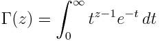
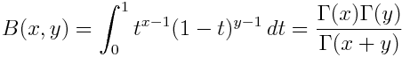 여기에 들어가는 $\Gamma(a)$는 감마 함수(Gamma function)
쫄지 마세요!
어차피 베타 함수의 역할은 normalizing constant
이미 구현된 계산 함수를 쓰면 됨ㅋ
국문 위키 http://ko.wikipedia.org/wiki/%EB%B2%A0%ED%83%80_%EB%B6%84%ED%8F%AC
Beta 분포를 왜 쓰냐면...
- 0에서 1 사이 값을 갖는 확률 변수에 대해 "수학적으로 깔끔하게" 확률을 매길 수 있다.
- 그렇다고 모든 경우의 수를 다 표현할 수 있는 건 아니지만...
- Bayesian update를 말도 안 되게 쉽게 할 수 있다!
In [50]:
''' building beta distribution '''
import numpy as np
from scipy.special import beta # beta function

def beta_pdf(x, a, b):
    return (x**(a-1)) *((1-x)**(b-1)) / (beta(a,b))
1.0
[ 1.  1.]
In [54]:
x = np.linspace(0,1,200)
p = beta_pdf(x,2,2)
plt.plot(x,p,'-')
plt.title('Beta distribution - Prior density')
plt.xlabel('x')
plt.ylabel('probability density')
Out[54]:
<matplotlib.text.Text at 0x7fe4919909d0>

In [58]:
''' a=b=1 gives uniform prior distribution '''
a = 1
b = 1

''' The Bayesian update '''
a += 140
b += 110
x = np.linspace(0,1,200)
p = beta_pdf(x,a,b)
plt.plot(x,p,'-')
plt.title('Beta distribution - Posterior density')
plt.xlabel('x')
plt.ylabel('probability density')
plt.figure()

''' comparison to the discrete prior case '''
PlotSuites([suite1])
kwargs = {'title':'Posterior from Uniform Prior', 'xlabel':'p(%)', 'ylabel':'probability mass'}
thinkplot.Show(**kwargs)

