Normalisation Demo - Prescriptions
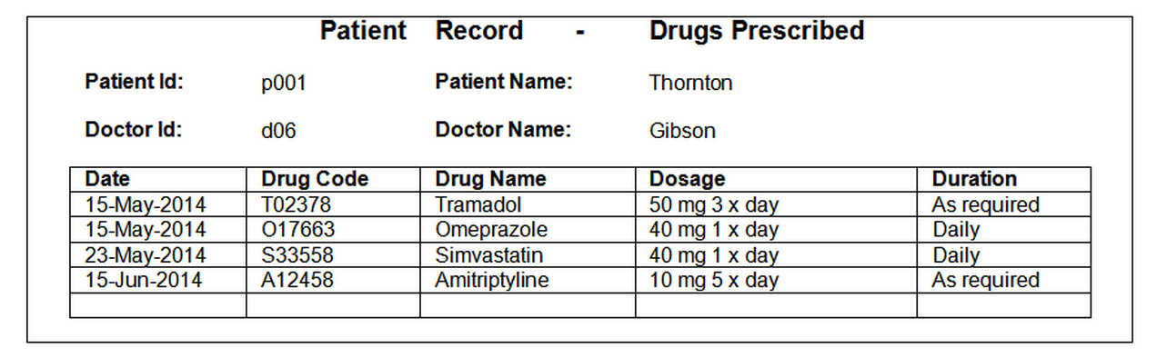
A worked example of how to normalise the example prescription data, using prescription data records of the following form:
import pandas as pd
Unnormalised Form (UNF)
#Read in the data file
df=pd.read_csv('data/normalisation-prescription.csv')
df
| patient_id | patient_name | doctor_id | doctor_name | date | drug_code | drug_name | dosage | duration | |
|---|---|---|---|---|---|---|---|---|---|
| 0 | p001 | Thornton | d06 | Gibson | 15-May-14 | T02378 | Tramadol | 50 mg 3 x day | As required |
| 1 | NaN | NaN | NaN | NaN | 15-May-14 | O17663 | Omeprazole | 40 mg 1 x day | Daily |
| 2 | NaN | NaN | NaN | NaN | 23-May-14 | S33558 | Simvastatin | 40 mg 1 x day | Daily |
| 3 | NaN | NaN | NaN | NaN | 15-Jun-14 | A12458 | Amitriptyline | 10 mg 5 x day | As required |
| 4 | p007 | Tennent | d07 | Paxton | 01-Jun-14 | C31319 | Ciprofloxacin | 500 mg 2 x day | 20 days |
| 5 | NaN | NaN | NaN | NaN | 01-Jun-14 | T05223 | Tamsulosin | 40 mg 1 x day | 20 days |
| 6 | NaN | NaN | NaN | NaN | 01-Jul-14 | S33558 | Simvastatin | 20 mg 1 x day | 6 weeks |
Note that there are cells in the table with null values that should actually be read as having the value of the previously populated cell.
Note that the contents of these empty cells is thus highly dependent on the order of the rows in the table. Maintaining such a table by hand in an spreadsheet could thus be prone to significant errors. If new precscription items are added to each patient's record at the bottom of their precscription list, it could be easy to make a mistake in making sure the prescription is added to the correct person's list, especially if the list is long and you can't accurately see whose list you are adding a new item too (for example, if their name has scrolled off the top of the page).
Let's tidy up the data by filing in the blanks. As the .fillna() documentation describes, the forward fill method (ffill) "can propagate [the] last valid observation forward to next valid [one]".
df.fillna(method='ffill', inplace=True)
df
| patient_id | patient_name | doctor_id | doctor_name | date | drug_code | drug_name | dosage | duration | |
|---|---|---|---|---|---|---|---|---|---|
| 0 | p001 | Thornton | d06 | Gibson | 15-May-14 | T02378 | Tramadol | 50 mg 3 x day | As required |
| 1 | p001 | Thornton | d06 | Gibson | 15-May-14 | O17663 | Omeprazole | 40 mg 1 x day | Daily |
| 2 | p001 | Thornton | d06 | Gibson | 23-May-14 | S33558 | Simvastatin | 40 mg 1 x day | Daily |
| 3 | p001 | Thornton | d06 | Gibson | 15-Jun-14 | A12458 | Amitriptyline | 10 mg 5 x day | As required |
| 4 | p007 | Tennent | d07 | Paxton | 01-Jun-14 | C31319 | Ciprofloxacin | 500 mg 2 x day | 20 days |
| 5 | p007 | Tennent | d07 | Paxton | 01-Jun-14 | T05223 | Tamsulosin | 40 mg 1 x day | 20 days |
| 6 | p007 | Tennent | d07 | Paxton | 01-Jul-14 | S33558 | Simvastatin | 20 mg 1 x day | 6 weeks |
First Normal Form (1NF)
To represent the data in 1NF we remove any repeating groups of data to separate relations, and choose a primary key for each new relation. A repeating group of data is defined as any attribute or group of attributes that may occur with multiple values for a single value of the primary key.
So what data elements repeat?
for c in df.columns:
    print(c,df[c].value_counts(),sep='\n',end='\n\n')
patient_id
p001    4
p007    3
dtype: int64

patient_name
Thornton    4
Tennent     3
dtype: int64

doctor_id
d06    4
d07    3
dtype: int64

doctor_name
Gibson    4
Paxton    3
dtype: int64

date
15-May-14    2
01-Jun-14    2
01-Jul-14    1
15-Jun-14    1
23-May-14    1
dtype: int64

drug_code
S33558    2
C31319    1
T02378    1
T05223    1
O17663    1
A12458    1
dtype: int64

drug_name
Simvastatin      2
Tramadol         1
Ciprofloxacin    1
Tamsulosin       1
Omeprazole       1
Amitriptyline    1
dtype: int64

dosage
40 mg 1 x day     3
500 mg 2 x day    1
20 mg 1 x day     1
10 mg 5 x day     1
50 mg 3 x day     1
dtype: int64

duration
As required    2
Daily          2
20 days        2
6 weeks        1
dtype: int64
By inspection, some of the columns appear to have similar structures, based on the counts of unique items.
For example, the patient_id, patient_name, doctor_id and doctor_name tables each contain two unique values, with 4 occurrences of one value and 3 of the other. Let's separate them out into another table.
df_1a=df[['patient_id', 'patient_name', 'doctor_id','doctor_name']]
df_1a
| patient_id | patient_name | doctor_id | doctor_name | |
|---|---|---|---|---|
| 0 | p001 | Thornton | d06 | Gibson |
| 1 | p001 | Thornton | d06 | Gibson |
| 2 | p001 | Thornton | d06 | Gibson |
| 3 | p001 | Thornton | d06 | Gibson |
| 4 | p007 | Tennent | d07 | Paxton |
| 5 | p007 | Tennent | d07 | Paxton |
| 6 | p007 | Tennent | d07 | Paxton |
We actually want to retain the unique combinations of these.
df_1a=df_1a.drop_duplicates()
df_1a
| patient_id | patient_name | doctor_id | doctor_name | |
|---|---|---|---|---|
| 0 | p001 | Thornton | d06 | Gibson |
| 4 | p007 | Tennent | d07 | Paxton |
We need to retain one of these columns as a key element in the actual prescriptions table. As the prescriptions are applied to patients, it perhaps makes sense to use a unique paitent identifier as the link which is to say, patient id. Let's create a new table by dropping the patient_name, doctor_id and doctor_name columns from the original table, but retaining the patient id column and the other columns relating to the prescription.
df_1b=df.drop(['patient_name', 'doctor_id','doctor_name'], 1)
df_1b
| patient_id | date | drug_code | drug_name | dosage | duration | |
|---|---|---|---|---|---|---|
| 0 | p001 | 15-May-14 | T02378 | Tramadol | 50 mg 3 x day | As required |
| 1 | p001 | 15-May-14 | O17663 | Omeprazole | 40 mg 1 x day | Daily |
| 2 | p001 | 23-May-14 | S33558 | Simvastatin | 40 mg 1 x day | Daily |
| 3 | p001 | 15-Jun-14 | A12458 | Amitriptyline | 10 mg 5 x day | As required |
| 4 | p007 | 01-Jun-14 | C31319 | Ciprofloxacin | 500 mg 2 x day | 20 days |
| 5 | p007 | 01-Jun-14 | T05223 | Tamsulosin | 40 mg 1 x day | 20 days |
| 6 | p007 | 01-Jul-14 | S33558 | Simvastatin | 20 mg 1 x day | 6 weeks |
As both new relations have an attribute in common, patient_id, the original relation can be recreated from these relations by performing a join operation on patient_id.
pd.merge(df_1a,df_1b,on='patient_id')
| patient_id | patient_name | doctor_id | doctor_name | date | drug_code | drug_name | dosage | duration | |
|---|---|---|---|---|---|---|---|---|---|
| 0 | p001 | Thornton | d06 | Gibson | 15-May-14 | T02378 | Tramadol | 50 mg 3 x day | As required |
| 1 | p001 | Thornton | d06 | Gibson | 15-May-14 | O17663 | Omeprazole | 40 mg 1 x day | Daily |
| 2 | p001 | Thornton | d06 | Gibson | 23-May-14 | S33558 | Simvastatin | 40 mg 1 x day | Daily |
| 3 | p001 | Thornton | d06 | Gibson | 15-Jun-14 | A12458 | Amitriptyline | 10 mg 5 x day | As required |
| 4 | p007 | Tennent | d07 | Paxton | 01-Jun-14 | C31319 | Ciprofloxacin | 500 mg 2 x day | 20 days |
| 5 | p007 | Tennent | d07 | Paxton | 01-Jun-14 | T05223 | Tamsulosin | 40 mg 1 x day | 20 days |
| 6 | p007 | Tennent | d07 | Paxton | 01-Jul-14 | S33558 | Simvastatin | 20 mg 1 x day | 6 weeks |
Second Normal Form (2NF)
In the first of the two 1NF relations shown above, the combination of patient_id, date and drug_code attributes together determine the dosage and duration attributes, but only drug_code determines drug_name. Thus, drug_name is removed from the relation, and drug_code and drug_name form a new relation, with drug_code as the primary key.
#Split out the drug code and drug name
df_2a=df_1b[['drug_code','drug_name']].drop_duplicates()
df_2a
| drug_code | drug_name | |
|---|---|---|
| 0 | T02378 | Tramadol |
| 1 | O17663 | Omeprazole |
| 2 | S33558 | Simvastatin |
| 3 | A12458 | Amitriptyline |
| 4 | C31319 | Ciprofloxacin |
| 5 | T05223 | Tamsulosin |
#Remove the drug name from table
df_2b=df_1b.drop(['drug_name'], 1)
df_2b
| patient_id | date | drug_code | dosage | duration | |
|---|---|---|---|---|---|
| 0 | p001 | 15-May-14 | T02378 | 50 mg 3 x day | As required |
| 1 | p001 | 15-May-14 | O17663 | 40 mg 1 x day | Daily |
| 2 | p001 | 23-May-14 | S33558 | 40 mg 1 x day | Daily |
| 3 | p001 | 15-Jun-14 | A12458 | 10 mg 5 x day | As required |
| 4 | p007 | 01-Jun-14 | C31319 | 500 mg 2 x day | 20 days |
| 5 | p007 | 01-Jun-14 | T05223 | 40 mg 1 x day | 20 days |
| 6 | p007 | 01-Jul-14 | S33558 | 20 mg 1 x day | 6 weeks |
As both new relations have an attribute in common, drug_code, the original relation can be recreated from these relations by performing a join operation on drug_code.
#Test the join
pd.merge(df_2a,df_2b,on='drug_code')
| drug_code | drug_name | patient_id | date | dosage | duration | |
|---|---|---|---|---|---|---|
| 0 | T02378 | Tramadol | p001 | 15-May-14 | 50 mg 3 x day | As required |
| 1 | O17663 | Omeprazole | p001 | 15-May-14 | 40 mg 1 x day | Daily |
| 2 | S33558 | Simvastatin | p001 | 23-May-14 | 40 mg 1 x day | Daily |
| 3 | S33558 | Simvastatin | p007 | 01-Jul-14 | 20 mg 1 x day | 6 weeks |
| 4 | A12458 | Amitriptyline | p001 | 15-Jun-14 | 10 mg 5 x day | As required |
| 5 | C31319 | Ciprofloxacin | p007 | 01-Jun-14 | 500 mg 2 x day | 20 days |
| 6 | T05223 | Tamsulosin | p007 | 01-Jun-14 | 40 mg 1 x day | 20 days |
Third Normal Form (3NF)
To represent the data in 3NF we remove any attributes that are not directly dependent upon the primary key to separate relations, and choose a primary key for each new relation.
In the second of the two 1NF relations shown above, the patient_name and doctor_id attributes are all directly dependent on patient_id but, doctor_name is directly dependent on doctor_id not patient_id. Therefore create a new relation from doctor_id and doctor_name where doctor_id is the primary key. The doctor_id remains in the original relation, as its value is determined by patient_id and where it acts as a foreign key referencing the new relation.
#Separate out the doctor and patient details
df_3a=df_1a[['doctor_id','doctor_name']]
df_3a
| doctor_id | doctor_name | |
|---|---|---|
| 0 | d06 | Gibson |
| 4 | d07 | Paxton |
df_3b=df_1a.drop(['doctor_name'],1)
df_3b
| patient_id | patient_name | doctor_id | |
|---|---|---|---|
| 0 | p001 | Thornton | d06 |
| 4 | p007 | Tennent | d07 |
As both new relations have an attribute in common, doctor_id, the original relation can be recreated from these relations by performing a join operation on doctor_id.
pd.merge(df_3a,df_3b,on='doctor_id')
| doctor_id | doctor_name | patient_id | patient_name | |
|---|---|---|---|---|
| 0 | d06 | Gibson | p001 | Thornton |
| 1 | d07 | Paxton | p007 | Tennent |
That's where the example stops. Don't we need to go a step further?
df_3c=df_3b[['patient_id','patient_name']]
df_3c
| patient_id | patient_name | |
|---|---|---|
| 0 | p001 | Thornton |
| 4 | p007 | Tennent |
df_3d=df_3b.drop(['patient_name'],1)
df_3d
| patient_id | doctor_id | |
|---|---|---|
| 0 | p001 | d06 |
| 4 | p007 | d07 |
Making a Function of It...
Looking at the steps abovem can we make a function to help perform some of the above operations?
def tableNorming(df,newTableCols,keyCol):
    df1=df[newTableCols].drop_duplicates()
    df2=df.drop(set(newTableCols)-set([keyCol]),1)
    return df1,df2
a,b=tableNorming(df,['patient_id', 'patient_name', 'doctor_id','doctor_name'],'patient_id')
a
| patient_id | patient_name | doctor_id | doctor_name | |
|---|---|---|---|---|
| 0 | p001 | Thornton | d06 | Gibson |
| 4 | p007 | Tennent | d07 | Paxton |
b
| patient_id | date | drug_code | drug_name | dosage | duration | |
|---|---|---|---|---|---|---|
| 0 | p001 | 15-May-14 | T02378 | Tramadol | 50 mg 3 x day | As required |
| 1 | p001 | 15-May-14 | O17663 | Omeprazole | 40 mg 1 x day | Daily |
| 2 | p001 | 23-May-14 | S33558 | Simvastatin | 40 mg 1 x day | Daily |
| 3 | p001 | 15-Jun-14 | A12458 | Amitriptyline | 10 mg 5 x day | As required |
| 4 | p007 | 01-Jun-14 | C31319 | Ciprofloxacin | 500 mg 2 x day | 20 days |
| 5 | p007 | 01-Jun-14 | T05223 | Tamsulosin | 40 mg 1 x day | 20 days |
| 6 | p007 | 01-Jul-14 | S33558 | Simvastatin | 20 mg 1 x day | 6 weeks |
Exercise - Invoice Data
Data from a dataset generated from invoice records taking the following form:
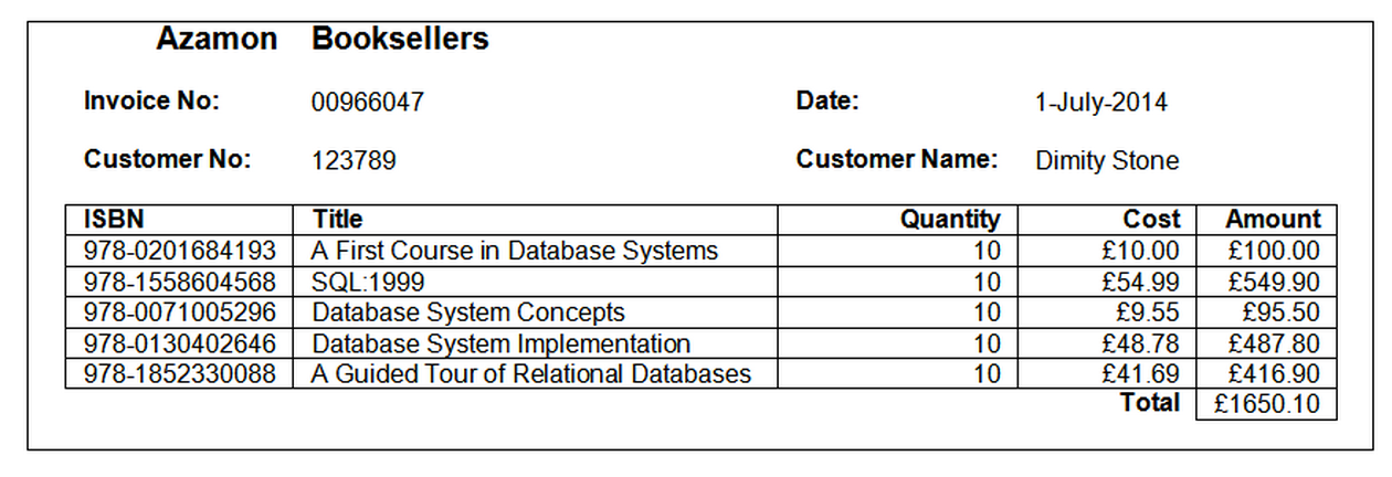
is presented in an unnormalised form:
#Read in the data file
ex1=pd.read_csv('data/normalisation-books.csv')
ex1
| invoice_no | date | customer_no | customer_name | isbn | title | quantity | cost | |
|---|---|---|---|---|---|---|---|---|
| 0 | 966047 | 01-Jul-14 | 123789 | Dimity Stone | 978-1292025827 | A First Course in Database Systems | 10 | £10.00 |
| 1 | NaN | NaN | NaN | NaN | 978-1558604568 | SQL:1999 | 10 | £54.99 |
| 2 | NaN | NaN | NaN | NaN | 978-0071005296 | Database System Concepts | 10 | £9.55 |
| 3 | NaN | NaN | NaN | NaN | 978-0130402646 | Database System Implementation | 10 | £48.78 |
| 4 | NaN | NaN | NaN | NaN | 978-1852330088 | A Guided Tour of Relational Databases | 10 | £41.69 |
| 5 | 966048 | 01-Jul-14 | 234678 | Roger Monk | 978-0071005296 | Database System Concepts | 1 | £9.55 |
| 6 | NaN | NaN | NaN | NaN | 978-0471141617 | Building the Data Warehouse | 1 | £9.55 |
| 7 | NaN | NaN | NaN | NaN | 978-1558604896 | Data Mining: Concepts and Techniques | 1 | £18.55 |
Clean the dataset as required and then put it into a set of normalised relations (tables) that avoid unnecessary duplication of data, and minimise the chances of update, deletion and addition anomalies.
Discussion
#Clean
ex1.fillna(method='ffill', inplace=True)
ex1
| invoice_no | date | customer_no | customer_name | isbn | title | quantity | cost | |
|---|---|---|---|---|---|---|---|---|
| 0 | 966047 | 01-Jul-14 | 123789 | Dimity Stone | 978-1292025827 | A First Course in Database Systems | 10 | £10.00 |
| 1 | 966047 | 01-Jul-14 | 123789 | Dimity Stone | 978-1558604568 | SQL:1999 | 10 | £54.99 |
| 2 | 966047 | 01-Jul-14 | 123789 | Dimity Stone | 978-0071005296 | Database System Concepts | 10 | £9.55 |
| 3 | 966047 | 01-Jul-14 | 123789 | Dimity Stone | 978-0130402646 | Database System Implementation | 10 | £48.78 |
| 4 | 966047 | 01-Jul-14 | 123789 | Dimity Stone | 978-1852330088 | A Guided Tour of Relational Databases | 10 | £41.69 |
| 5 | 966048 | 01-Jul-14 | 234678 | Roger Monk | 978-0071005296 | Database System Concepts | 1 | £9.55 |
| 6 | 966048 | 01-Jul-14 | 234678 | Roger Monk | 978-0471141617 | Building the Data Warehouse | 1 | £9.55 |
| 7 | 966048 | 01-Jul-14 | 234678 | Roger Monk | 978-1558604896 | Data Mining: Concepts and Techniques | 1 | £18.55 |
#Review the data
for c in ex1.columns:
    print(c,ex1[c].value_counts(),sep='\n',end='\n\n')
invoice_no
966047    5
966048    3
dtype: int64

date
01-Jul-14    8
dtype: int64

customer_no
123789    5
234678    3
dtype: int64

customer_name
Dimity Stone    5
Roger Monk      3
dtype: int64

isbn
978-0071005296    2
978-1558604896    1
978-0471141617    1
978-0130402646    1
978-1292025827    1
978-1852330088    1
978-1558604568    1
dtype: int64

title
Database System Concepts                 2
A Guided Tour of Relational Databases    1
Building the Data Warehouse              1
Data Mining: Concepts and Techniques     1
Database System Implementation           1
A First Course in Database Systems       1
SQL:1999                                 1
dtype: int64

quantity
10    5
1     3
dtype: int64

cost
£9.55     3
£18.55    1
£48.78    1
£10.00    1
£41.69    1
£54.99    1
dtype: int64
If we were to simply inspect the unique counts, they might suggest that the invoice_no, customer_no, customer_name and quantity columns might share common sets of values as a repeating group. Looking at the column names and values, as well as the original invoice, we might anticipate that there is a meaningful relation between customer_no and customer_name, that an invoice_no relates to a particular transaction with a particular customer on a particular date, and the quantity is actually an independent value relating to the individual book purchase transactions detailed by a particular invoice.
#Convert to 1NF
ex1_1a,ex1_1b=tableNorming(ex1,['invoice_no', 'customer_no', 'customer_name','date'],'invoice_no')
ex1_1a
| invoice_no | customer_no | customer_name | date | |
|---|---|---|---|---|
| 0 | 966047 | 123789 | Dimity Stone | 01-Jul-14 |
| 5 | 966048 | 234678 | Roger Monk | 01-Jul-14 |
ex1_1b
| invoice_no | isbn | title | quantity | cost | |
|---|---|---|---|---|---|
| 0 | 966047 | 978-1292025827 | A First Course in Database Systems | 10 | £10.00 |
| 1 | 966047 | 978-1558604568 | SQL:1999 | 10 | £54.99 |
| 2 | 966047 | 978-0071005296 | Database System Concepts | 10 | £9.55 |
| 3 | 966047 | 978-0130402646 | Database System Implementation | 10 | £48.78 |
| 4 | 966047 | 978-1852330088 | A Guided Tour of Relational Databases | 10 | £41.69 |
| 5 | 966048 | 978-0071005296 | Database System Concepts | 1 | £9.55 |
| 6 | 966048 | 978-0471141617 | Building the Data Warehouse | 1 | £9.55 |
| 7 | 966048 | 978-1558604896 | Data Mining: Concepts and Techniques | 1 | £18.55 |
#Test
pd.merge(ex1_1a,ex1_1b,on='invoice_no')
| invoice_no | customer_no | customer_name | date | isbn | title | quantity | cost | |
|---|---|---|---|---|---|---|---|---|
| 0 | 966047 | 123789 | Dimity Stone | 01-Jul-14 | 978-1292025827 | A First Course in Database Systems | 10 | £10.00 |
| 1 | 966047 | 123789 | Dimity Stone | 01-Jul-14 | 978-1558604568 | SQL:1999 | 10 | £54.99 |
| 2 | 966047 | 123789 | Dimity Stone | 01-Jul-14 | 978-0071005296 | Database System Concepts | 10 | £9.55 |
| 3 | 966047 | 123789 | Dimity Stone | 01-Jul-14 | 978-0130402646 | Database System Implementation | 10 | £48.78 |
| 4 | 966047 | 123789 | Dimity Stone | 01-Jul-14 | 978-1852330088 | A Guided Tour of Relational Databases | 10 | £41.69 |
| 5 | 966048 | 234678 | Roger Monk | 01-Jul-14 | 978-0071005296 | Database System Concepts | 1 | £9.55 |
| 6 | 966048 | 234678 | Roger Monk | 01-Jul-14 | 978-0471141617 | Building the Data Warehouse | 1 | £9.55 |
| 7 | 966048 | 234678 | Roger Monk | 01-Jul-14 | 978-1558604896 | Data Mining: Concepts and Techniques | 1 | £18.55 |
#Convert to 2NF
#In ex1_1b, the combination of invoice_no and isbn attributes together determine the quantity attribute.
# Only isbn determines cost. cost is removed from the relation, and isbn and cost form a new relation, with isbn as key.

ex1_2a,ex1_2b=tableNorming(ex1_1b,['isbn', 'title', 'cost'],'isbn')
ex1_2a
| isbn | title | cost | |
|---|---|---|---|
| 0 | 978-1292025827 | A First Course in Database Systems | £10.00 |
| 1 | 978-1558604568 | SQL:1999 | £54.99 |
| 2 | 978-0071005296 | Database System Concepts | £9.55 |
| 3 | 978-0130402646 | Database System Implementation | £48.78 |
| 4 | 978-1852330088 | A Guided Tour of Relational Databases | £41.69 |
| 6 | 978-0471141617 | Building the Data Warehouse | £9.55 |
| 7 | 978-1558604896 | Data Mining: Concepts and Techniques | £18.55 |
ex1_2b
| invoice_no | isbn | quantity | |
|---|---|---|---|
| 0 | 966047 | 978-1292025827 | 10 |
| 1 | 966047 | 978-1558604568 | 10 |
| 2 | 966047 | 978-0071005296 | 10 |
| 3 | 966047 | 978-0130402646 | 10 |
| 4 | 966047 | 978-1852330088 | 10 |
| 5 | 966048 | 978-0071005296 | 1 |
| 6 | 966048 | 978-0471141617 | 1 |
| 7 | 966048 | 978-1558604896 | 1 |
#Test
pd.merge(ex1_2a,ex1_2b,on='isbn')
| isbn | title | cost | invoice_no | quantity | |
|---|---|---|---|---|---|
| 0 | 978-1292025827 | A First Course in Database Systems | £10.00 | 966047 | 10 |
| 1 | 978-1558604568 | SQL:1999 | £54.99 | 966047 | 10 |
| 2 | 978-0071005296 | Database System Concepts | £9.55 | 966047 | 10 |
| 3 | 978-0071005296 | Database System Concepts | £9.55 | 966048 | 1 |
| 4 | 978-0130402646 | Database System Implementation | £48.78 | 966047 | 10 |
| 5 | 978-1852330088 | A Guided Tour of Relational Databases | £41.69 | 966047 | 10 |
| 6 | 978-0471141617 | Building the Data Warehouse | £9.55 | 966048 | 1 |
| 7 | 978-1558604896 | Data Mining: Concepts and Techniques | £18.55 | 966048 | 1 |
#Convert to 3NF
#In ex1_1a, the date and customer_no attributes are all directly dependent on invoice_no
#customer_name is directly dependent on customer_no not invoice_no.
#Therefore create a new relation from customer_no and customer_name where customer_no is the primary key.
#The customer_no remains in the original relation as a foreign key, as its value is determined by invoice_no

ex1_3a,ex1_3b=tableNorming(ex1_1a,['customer_no', 'customer_name'],'customer_no')
ex1_3a
| customer_no | customer_name | |
|---|---|---|
| 0 | 123789 | Dimity Stone |
| 5 | 234678 | Roger Monk |
ex1_3b
| invoice_no | customer_no | date | |
|---|---|---|---|
| 0 | 966047 | 123789 | 01-Jul-14 |
| 5 | 966048 | 234678 | 01-Jul-14 |
#Test
pd.merge(ex1_3a,ex1_3b,on='customer_no')
| customer_no | customer_name | invoice_no | date | |
|---|---|---|---|---|
| 0 | 123789 | Dimity Stone | 966047 | 01-Jul-14 |
| 1 | 234678 | Roger Monk | 966048 | 01-Jul-14 |
Exercise
ex3=pd.read_csv('data/normalisation-authors.csv')
ex3
| isbn | title | authors | cost | |
|---|---|---|---|---|
| 0 | 978-1292025827 | A First Course in Database Systems | Jeffrey D Ullman, Jennifer Widom | £10.00 |
| 1 | 978-1558604568 | SQL:1999 | Jim Melton, Alan R Simon | £54.99 |
| 2 | 978-0071005296 | Database System Concepts | Henry F Korth, Abraham Silberschatz | £9.55 |
| 3 | 978-0130402646 | Database System Implementation | Hector Garcia-Molina, Jeffrey D Ullman, Jennif... | £48.78 |
| 4 | 978-1852330088 | A Guided Tour of Relational Databases | Mark Levene, George Loizou | £41.69 |
| 5 | 978-0471141617 | Building the Data Warehouse | William H Inmon | £9.55 |
| 6 | 978-1558604896 | Data Mining: Concepts and Techniques | Jiawei Han, Micheline Kamber | £18.55 |
To be able to list books by author, we need to reshape this dataset by splitting on the authors column. In the original table, authors are essentially specified in a comma separated list.
#Sort of via http://stackoverflow.com/a/12681217/454773
ex3_authors=pd.concat([pd.DataFrame({'isbn':row['isbn'], 'author':row['authors'].split(',') })
                    for _, row in ex3.iterrows()])
ex3_authors
| author | isbn | |
|---|---|---|
| 0 | Jeffrey D Ullman | 978-1292025827 |
| 1 | Jennifer Widom | 978-1292025827 |
| 0 | Jim Melton | 978-1558604568 |
| 1 | Alan R Simon | 978-1558604568 |
| 0 | Henry F Korth | 978-0071005296 |
| 1 | Abraham Silberschatz | 978-0071005296 |
| 0 | Hector Garcia-Molina | 978-0130402646 |
| 1 | Jeffrey D Ullman | 978-0130402646 |
| 2 | Jennifer Widom | 978-0130402646 |
| 0 | Mark Levene | 978-1852330088 |
| 1 | George Loizou | 978-1852330088 |
| 0 | William H Inmon | 978-0471141617 |
| 0 | Jiawei Han | 978-1558604896 |
| 1 | Micheline Kamber | 978-1558604896 |
ex3_books=ex3.drop('authors',1)
ex3_books
| isbn | title | cost | |
|---|---|---|---|
| 0 | 978-1292025827 | A First Course in Database Systems | £10.00 |
| 1 | 978-1558604568 | SQL:1999 | £54.99 |
| 2 | 978-0071005296 | Database System Concepts | £9.55 |
| 3 | 978-0130402646 | Database System Implementation | £48.78 |
| 4 | 978-1852330088 | A Guided Tour of Relational Databases | £41.69 |
| 5 | 978-0471141617 | Building the Data Warehouse | £9.55 |
| 6 | 978-1558604896 | Data Mining: Concepts and Techniques | £18.55 |