Gradient Boosted Regression Trees
Scikit-learn
- Easy-to-use Machine Learning toolkit
- Classical, well-established machine learning algorithms
- BSD 3 license
Estimator
"An estimator is any object that learns from data; it may be a classification, regression or clustering algorithm or a transformer that extracts/filters useful features from raw data."
class Estimator(object):

    def fit(self, X, y=None):
        """Fits estimator to data. """
        # set state of ``self``
        return self

    def predict(self, X):
        """Predict response of ``X``. """
        # compute predictions ``pred``
        return pred
Scikit-learn provides two estimators for gradient boosting: GradientBoostingClassifier and GradientBoostingRegressor, both are located in the sklearn.ensemble package:
from sklearn.ensemble import GradientBoostingClassifier
from sklearn.ensemble import GradientBoostingRegressor
Estimators support arguments to control the fitting behaviour -- these arguments are often called hyperparameters. Among the most important ones for GBRT are:
- number of regression trees (
n_estimators) - depth of each individual tree (
max_depth) - loss function (
loss)
For example if you want to fit a regression model with 100 trees of depth 3 using least-squares:
est = GradientBoostingRegressor(n_estimators=100, max_depth=3, loss='ls')
est?
Here is an self-contained example that shows how to fit a GradientBoostingClassifier to a synthetic dataset:
from sklearn.datasets import make_hastie_10_2
from sklearn.cross_validation import train_test_split

# generate synthetic data from ESLII - Example 10.2
X, y = make_hastie_10_2(n_samples=5000)
X_train, X_test, y_train, y_test = train_test_split(X, y)

# fit estimator
est = GradientBoostingClassifier(n_estimators=200, max_depth=3)
est.fit(X_train, y_train)

# predict class labels
pred = est.predict(X_test)

# score on test data (accuracy)
acc = est.score(X_test, y_test)
print('ACC: %.4f' % acc)

# predict class probabilities
est.predict_proba(X_test)[0]
ACC: 0.9224
array([ 0.74435614, 0.25564386])
The state of the estimator is stored in instance attributes that have a trailing underscore ('_'). For example, the sequence of regression trees (DecisionTreeRegressor objects) is stored in est.estimators_:
est.estimators_[0, 0]
DecisionTreeRegressor(compute_importances=None,
           criterion=<sklearn.tree._tree.FriedmanMSE object at 0x3e4eb28>,
           max_depth=3, max_features=None, max_leaf_nodes=None,
           min_density=None, min_samples_leaf=1, min_samples_split=2,
           random_state=<mtrand.RandomState object at 0x7feca45d6660>,
           splitter=<sklearn.tree._tree.PresortBestSplitter object at 0x3da15b0>)
%pylab inline
import numpy as np
from sklearn.cross_validation import train_test_split

FIGSIZE = (11, 7)

def ground_truth(x):
    """Ground truth -- function to approximate"""
    return x * np.sin(x) + np.sin(2 * x)

def gen_data(n_samples=200):
    """generate training and testing data"""
    np.random.seed(15)
    X = np.random.uniform(0, 10, size=n_samples)[:, np.newaxis]
    y = ground_truth(X.ravel()) + np.random.normal(scale=2, size=n_samples)
    train_mask = np.random.randint(0, 2, size=n_samples).astype(np.bool)
    X_train, X_test, y_train, y_test = train_test_split(X, y, test_size=0.2, random_state=3)
    return X_train, X_test, y_train, y_test

X_train, X_test, y_train, y_test = gen_data(100)

# plot ground truth
x_plot = np.linspace(0, 10, 500)

def plot_data(alpha=0.4, s=20):
    fig = plt.figure(figsize=FIGSIZE)
    gt = plt.plot(x_plot, ground_truth(x_plot), alpha=alpha, label='ground truth')

    # plot training and testing data
    plt.scatter(X_train, y_train, s=s, alpha=alpha)
    plt.scatter(X_test, y_test, s=s, alpha=alpha, color='red')
    plt.xlim((0, 10))
    plt.ylabel('y')
    plt.xlabel('x')

annotation_kw = {'xycoords': 'data', 'textcoords': 'data',
                 'arrowprops': {'arrowstyle': '->', 'connectionstyle': 'arc'}}

plot_data()
Populating the interactive namespace from numpy and matplotlib

Regression Trees
max_depthargument controlls the depth of the tree- The deeper the tree the more variance can be explained
from sklearn.tree import DecisionTreeRegressor
plot_data()
est = DecisionTreeRegressor(max_depth=1).fit(X_train, y_train)
plt.plot(x_plot, est.predict(x_plot[:, np.newaxis]),
         label='RT max_depth=1', color='g', alpha=0.9, linewidth=2)

est = DecisionTreeRegressor(max_depth=3).fit(X_train, y_train)
plt.plot(x_plot, est.predict(x_plot[:, np.newaxis]),
         label='RT max_depth=3', color='g', alpha=0.7, linewidth=1)

plt.legend(loc='upper left')
<matplotlib.legend.Legend at 0x4ab22d0>

Function approximation with Gradient Boosting
n_estimatorsargument controls the number of treesstaged_predictmethod allows us to step through predictions as we add more trees
from itertools import islice

plot_data()
est = GradientBoostingRegressor(n_estimators=1000, max_depth=1, learning_rate=1.0)
est.fit(X_train, y_train)

ax = plt.gca()
first = True

# step through prediction as we add 10 more trees.
for pred in islice(est.staged_predict(x_plot[:, np.newaxis]), 0, est.n_estimators, 10):
    plt.plot(x_plot, pred, color='r', alpha=0.2)
    if first:
        ax.annotate('High bias - low variance', xy=(x_plot[x_plot.shape[0] // 2],
                                                    pred[x_plot.shape[0] // 2]),
                                                    xytext=(4, 4), **annotation_kw)
        first = False

pred = est.predict(x_plot[:, np.newaxis])
plt.plot(x_plot, pred, color='r', label='GBRT max_depth=1')
ax.annotate('Low bias - high variance', xy=(x_plot[x_plot.shape[0] // 2],
                                            pred[x_plot.shape[0] // 2]),
                                            xytext=(6.25, -6), **annotation_kw)
plt.legend(loc='upper left')
<matplotlib.legend.Legend at 0x5265390>

Model complexity
- The number of trees and the depth of the individual trees control model complexity
- Model complexity comes at a price: overfitting
Deviance plot
- Diagnostic to determine if model is overfitting
- Plots the training/testing error (deviance) as a function of the number of trees (=model complexity)
- Training error (deviance) is stored in
est.train_score_ - Test error is computed using
est.staged_predict
def deviance_plot(est, X_test, y_test, ax=None, label='', train_color='#2c7bb6',
                  test_color='#d7191c', alpha=1.0, ylim=(0, 10)):
    """Deviance plot for ``est``, use ``X_test`` and ``y_test`` for test error. """
    n_estimators = len(est.estimators_)
    test_dev = np.empty(n_estimators)

    for i, pred in enumerate(est.staged_predict(X_test)):
       test_dev[i] = est.loss_(y_test, pred)

    if ax is None:
        fig = plt.figure(figsize=FIGSIZE)
        ax = plt.gca()

    ax.plot(np.arange(n_estimators) + 1, test_dev, color=test_color, label='Test %s' % label,
             linewidth=2, alpha=alpha)
    ax.plot(np.arange(n_estimators) + 1, est.train_score_, color=train_color,
             label='Train %s' % label, linewidth=2, alpha=alpha)
    ax.set_ylabel('Error')
    ax.set_xlabel('n_estimators')
    ax.set_ylim(ylim)
    return test_dev, ax

test_dev, ax = deviance_plot(est, X_test, y_test)
ax.legend(loc='upper right')

# add some annotations
ax.annotate('Lowest test error', xy=(test_dev.argmin() + 1, test_dev.min() + 0.02),
            xytext=(150, 3.5), **annotation_kw)

ann = ax.annotate('', xy=(800, test_dev[799]),  xycoords='data',
                  xytext=(800, est.train_score_[799]), textcoords='data',
                  arrowprops={'arrowstyle': '<->'})
ax.text(810, 3.5, 'train-test gap')
<matplotlib.text.Text at 0x55f4150>

Overfitting
- Model has too much capacity and starts fitting the idiosyncracies of the training data
- Indicated by a large gap between train and test error
- GBRT provides a number of knobs to control overfitting
def fmt_params(params):
    return ", ".join("{0}={1}".format(key, val) for key, val in params.iteritems())

fig = plt.figure(figsize=FIGSIZE)
ax = plt.gca()
for params, (test_color, train_color) in [({}, ('#d7191c', '#2c7bb6')),
                                          ({'min_samples_leaf': 3}, ('#fdae61', '#abd9e9'))]:
    est = GradientBoostingRegressor(n_estimators=1000, max_depth=1,
                                    learning_rate=1.0)
    est.set_params(**params)
    est.fit(X_train, y_train)
    test_dev, ax = deviance_plot(est, X_test, y_test, ax=ax, label=fmt_params(params),
                                 train_color=train_color, test_color=test_color)

ax.annotate('Higher bias', xy=(900, est.train_score_[899]), xytext=(600, 3), **annotation_kw)
ax.annotate('Lower variance', xy=(900, test_dev[899]), xytext=(600, 3.5), **annotation_kw)
plt.legend(loc='upper right')
<matplotlib.legend.Legend at 0x4f42dd0>

Shrinkage
- Slow learning by shrinking the predictions of each tree by some small scalar (
learning_rate) - A lower
learning_raterequires a higher number ofn_estimators - Its a trade-off between runtime against accuracy.
fig = plt.figure(figsize=FIGSIZE)
ax = plt.gca()
for params, (test_color, train_color) in [({}, ('#d7191c', '#2c7bb6')),
                                          ({'learning_rate': 0.1},
                                           ('#fdae61', '#abd9e9'))]:
    est = GradientBoostingRegressor(n_estimators=1000, max_depth=1, learning_rate=1.0)
    est.set_params(**params)
    est.fit(X_train, y_train)

    test_dev, ax = deviance_plot(est, X_test, y_test, ax=ax, label=fmt_params(params),
                                 train_color=train_color, test_color=test_color)

ax.annotate('Requires more trees', xy=(200, est.train_score_[199]),
            xytext=(300, 1.75), **annotation_kw)
ax.annotate('Lower test error', xy=(900, test_dev[899]),
            xytext=(600, 1.75), **annotation_kw)
plt.legend(loc='upper right')
<matplotlib.legend.Legend at 0x5c8bd50>

Stochastic Gradient Boosting
- Subsampling the training set before growing each tree (
subsample) - Subsampling the features before finding the best split node (
max_features) - Latter usually works better if there is a sufficient large number of features
fig = plt.figure(figsize=FIGSIZE)
ax = plt.gca()
for params, (test_color, train_color) in [({}, ('#d7191c', '#2c7bb6')),
                                          ({'learning_rate': 0.1, 'subsample': 0.5},
                                           ('#fdae61', '#abd9e9'))]:
    est = GradientBoostingRegressor(n_estimators=1000, max_depth=1, learning_rate=1.0,
                                    random_state=1)
    est.set_params(**params)
    est.fit(X_train, y_train)
    test_dev, ax = deviance_plot(est, X_test, y_test, ax=ax, label=fmt_params(params),
                                 train_color=train_color, test_color=test_color)

ax.annotate('Even lower test error', xy=(400, test_dev[399]),
            xytext=(500, 3.0), **annotation_kw)

est = GradientBoostingRegressor(n_estimators=1000, max_depth=1, learning_rate=1.0,
                                subsample=0.5)
est.fit(X_train, y_train)
test_dev, ax = deviance_plot(est, X_test, y_test, ax=ax, label=fmt_params({'subsample': 0.5}),
                             train_color='#abd9e9', test_color='#fdae61', alpha=0.5)
ax.annotate('Subsample alone does poorly', xy=(300, test_dev[299]),
            xytext=(500, 5.5), **annotation_kw)
plt.legend(loc='upper right', fontsize='small')
<matplotlib.legend.Legend at 0x5490d90>

Hyperparameter tuning
I usually follow this recipe to tune the hyperparameters:
- Pick
n_estimatorsas large as (computationally) possible (e.g. 3000) - Tune
max_depth,learning_rate,min_samples_leaf, andmax_featuresvia grid search - Increase
n_estimatorseven more and tunelearning_rateagain holding the other parameters fixed
from sklearn.grid_search import GridSearchCV

param_grid = {'learning_rate': [0.1, 0.01, 0.001],
              'max_depth': [4, 6],
              'min_samples_leaf': [3, 5]  ## depends on the nr of training examples
              # 'max_features': [1.0, 0.3, 0.1] ## not possible in our example (only 1 fx)
              }

est = GradientBoostingRegressor(n_estimators=3000)
# this may take some minutes
gs_cv = GridSearchCV(est, param_grid, scoring='mean_squared_error', n_jobs=4).fit(X_train, y_train)

# best hyperparameter setting
print('Best hyperparameters: %r' % gs_cv.best_params_)
Best hyperparameters: {'learning_rate': 0.001, 'max_depth': 6, 'min_samples_leaf': 5}
# refit model on best parameters
est.set_params(**gs_cv.best_params_)
est.fit(X_train, y_train)

# plot the approximation
plot_data()
plt.plot(x_plot, est.predict(x_plot[:, np.newaxis]), color='r', linewidth=2)
[<matplotlib.lines.Line2D at 0x4c21810>]

Caution: Hyperparameters interact with each other (learning_rate and n_estimators, learning_rate and subsample, max_depth and max_features).
See G. Ridgeway, "Generalized boosted models: A guide to the gbm package", 2005
Use-case: California Housing

- Predict the median house value for census block groups in California
- 20.000 groups, 8 features: median income, average house age, latitude, longitude, ...
- Mean Absolute Error on 80-20 train-test split
from sklearn.datasets.california_housing import fetch_california_housing

cal_housing = fetch_california_housing()

# split 80/20 train-test
X_train, X_test, y_train, y_test = train_test_split(cal_housing.data,
                                                    cal_housing.target,
                                                    test_size=0.2,
                                                    random_state=1)
names = cal_housing.feature_names
Challenges
- heterogenous features (different scales and distributions, see plot below)
- non-linear feature interactions (interaction: latitude and longitude)
- extreme responses (robust regression techniques)
import pandas as pd
X_df = pd.DataFrame(data=X_train, columns=names)
X_df['MedHouseVal'] = y_train
_ = X_df.hist(column=['Latitude', 'Longitude', 'MedInc', 'MedHouseVal'], figsize=FIGSIZE)

Evaluation
- GBRT vs RandomForest vs SVM vs Ridge Regression
import time
from collections import defaultdict
from sklearn.metrics import mean_absolute_error
from sklearn.linear_model import Ridge
from sklearn.ensemble import RandomForestRegressor
from sklearn.pipeline import Pipeline
from sklearn.preprocessing import StandardScaler
from sklearn.dummy import DummyRegressor
from sklearn.svm import SVR

res = defaultdict(dict)

def benchmark(est, name=None):
    if not name:
        name = est.__class__.__name__
    t0 = time.clock()
    est.fit(X_train, y_train)
    res[name]['train_time'] = time.clock() - t0
    t0 = time.clock()
    pred = est.predict(X_test)
    res[name]['test_time'] = time.clock() - t0
    res[name]['MAE'] = mean_absolute_error(y_test, pred)
    return est

benchmark(DummyRegressor())
benchmark(Ridge(alpha=0.0001, normalize=True))
benchmark(Pipeline([('std', StandardScaler()),
                    ('svr', SVR(kernel='rbf', C=10.0, gamma=0.1, tol=0.001))]), name='SVR')
benchmark(RandomForestRegressor(n_estimators=100, max_features=5, random_state=0,
                                bootstrap=False, n_jobs=4))
est = benchmark(GradientBoostingRegressor(n_estimators=500, max_depth=4, learning_rate=0.1,
                                          loss='huber', min_samples_leaf=3,
                                          random_state=0))

res_df = pd.DataFrame(data=res).T
res_df[['train_time', 'test_time', 'MAE']].sort('MAE', ascending=False)
| train_time | test_time | MAE | |
|---|---|---|---|
| DummyRegressor | 0.00 | 0.00 | 0.909090 |
| Ridge | 0.02 | 0.00 | 0.532860 |
| SVR | 89.90 | 6.63 | 0.379575 |
| RandomForestRegressor | 74.73 | 0.50 | 0.318885 |
| GradientBoostingRegressor | 45.76 | 0.15 | 0.300638 |
Exercise
The above GradientBoostingRegressor is not properly tuned for this dataset. Diagnose the current model and find more appropriate hyperparameter settings.
Hint: check whether you are in the high-bias or high-variance regime
# diagnose the model
test_dev, ax = deviance_plot(est, X_test, y_test, ylim=(0, 1.0))

## modify the hyperparameters
#tuned_est = benchmark(GradientBoostingRegressor(n_estimators=500, max_depth=4, learning_rate=0.1,
#                                                loss='huber', random_state=0, verbose=1))

## print results
#res_df = pd.DataFrame(data=res).T
#res_df[['train_time', 'test_time', 'MAE']].sort('MAE', ascending=False)
Feature importance
- What are the important features and how do they contribute in predicting the target response?
- Derived from the regression trees
- Can be accessed via the attribute
est.feature_importances_
fx_imp = pd.Series(est.feature_importances_, index=names)
fx_imp /= fx_imp.max()  # normalize
fx_imp.sort()
fx_imp.plot(kind='barh', figsize=FIGSIZE)
<matplotlib.axes.AxesSubplot at 0x85a2550>

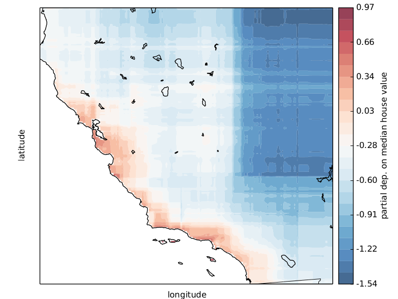
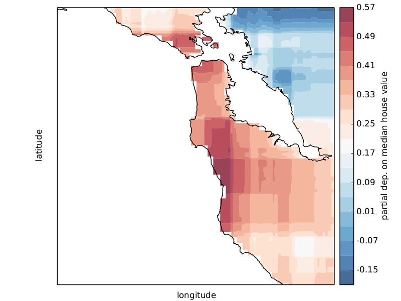
Partial dependence
- Relationship between the response and a set of features, marginalizing over all other features
- Intuitively: expected response as a function of the features we conditioned on
from sklearn.ensemble.partial_dependence import plot_partial_dependence

features = ['MedInc', 'AveOccup', 'HouseAge',
            ('AveOccup', 'HouseAge')]
fig, axs = plot_partial_dependence(est, X_train, features, feature_names=names,
                                   n_cols=2, figsize=FIGSIZE)

Scikit-learn provides a convenience function to create such plots and a low-level function that you can use to create custom partial dependence plots (e.g. map overlays or 3d plots). More detailed information can be found here.
df = pd.DataFrame(data={'icao': ['CRJ2', 'A380', 'B737', 'B737']})
# ordinal encoding
df_enc = pd.DataFrame(data={'icao': np.unique(df.icao,
                      return_inverse=True)[1]})
X = np.asfortranarray(df_enc.values, dtype=np.float32)
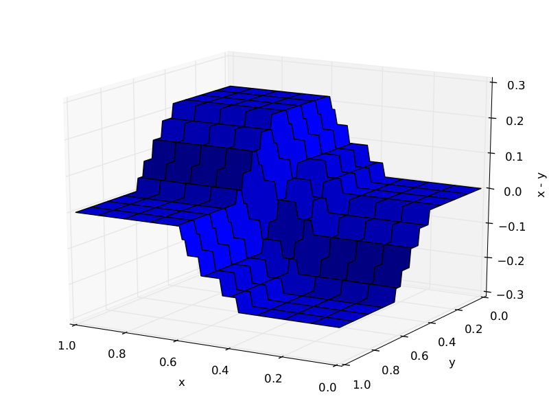
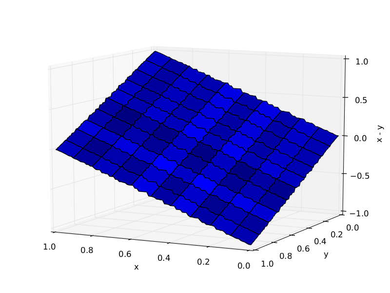
Feature interactions
GBRT automatically detects feature interactions but often explicit interactions help.
Trees required to approximate $X_1 - X_2$: 10 (left), 1000 (right)
Summary
- Flexible non-parametric classification and regression technique
- Applicable to a variety of problems
- Solid, battle-worn implementation in scikit-learn