%%html
<link rel="stylesheet" href="static/hyrule.css" type="text/css">
Relational Databases; SQL syntax
Objectives
- Review the context of denormalized vs normalized data in relational databases
- Compare and contrast SQL syntax to pandas (and when we should use what)
- Gain insight behind advanced database useage and defined functions in postgres.
Computer setup
In order to connect to the database we're using on ec2, we need psycopg2 installed in our Anaconda Python.
Try these routes first:
MAC: conda install -c https://conda.binstar.org/alefnula psycopg2
PC: conda install -c https://conda.binstar.org/topper psycopg2-windows
If you have issues, try directly installing with pip:
MAC: anaconda/bin/pip install psycopg2
PC: anaconda\pip.exe install psycopg2
If you're still having issues (mac folks), please consult here for additional help, but only IF you are running into dylib errors.
Parameters for connecting to the database will be given via Slack.
Class Notes
What are databases?
Databases are a structured data source optimized for efficient retrieval and storage.
- structured: we have to pre-define organization strategy
- retrieval: the ability to read data out
- storage: the ability to write data and save it
What is a relational database?
Relational databases are traditionally organized in the following manner:
- A database has tables which represent individual entities or objects.
- Tables have predefined schema – rules that tell it what the data will look like.
Each table should have a primary key column: a unique identifier for that row. Additionally, each table can have a foreign key column: an id that links this to another table.
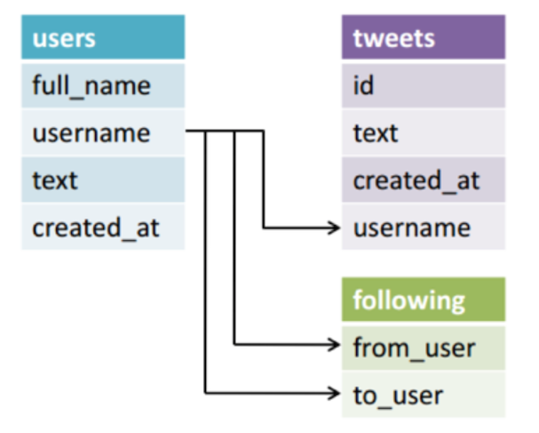
In a normalized schema, tables are designed to be thin in order to minimize:
- The amount of repeated information
- The amount of bytes stored
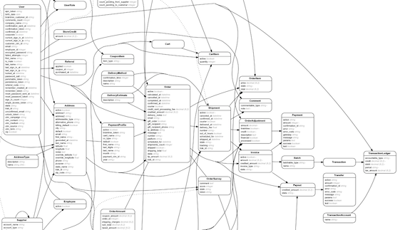 _Case in point; here is a relational diagram of a typical ecommerce platform_
What if we had designed the database to look this way with one table?
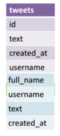
- Repeated information is increased; the user information is repeated in each row.
- There is increased text storage (text bytes are larger than integer bytes)
- There is no need to join!
The tradeoff between normalized and denormalized data is speed vs storage. Storage (for the most part) is the same everywhere.. so let's focus on the speed side. Speed breaks down into read speed and write speed.
Of the two data views:
- Which would we believe to be slower to read but faster to write?
- Which would we believe to be slower to write but faster to read?
SQL syntax
SQL (structured query language) is a query language for loading, retrieving, and updating data in relational databases. Most commonly used SQL databases include:
- Oracle and MySQL
- SQL Server
- PostgreSQL
The SQL-like structure is also heavily borrowed in large scale data languages and platforms:
- Apache Hive
- Apache Drill (based on Google's Dremel)
- Spark SQL
So it is important to learn the basics that fit across all platforms!
Good syntax
While companies and data teams end up developing their own sense of SQL style, those new to SQL should adopt at least the following style:
- Keywords are upper case and begin new lines
- fields in their own lines
- continuations are indented
This will be explained as we go through examples below. To help make some connections, there will be some python code blocks using pandas syntax to do similar statements to the SQL queries. They'll be labeled *pandas* and *end_pandas* to clarify where those are.
SELECT
Basic usecase for pulling data from the database.
SELECT
    col1,
    col2
FROM table
WHERE [some condition];
Example
SELECT
    poll_title,
    poll_date
FROM polls
WHERE romney_pct > obama_pct;
*pandas*
polls[polls.romney_pct > polls.obama_pct][['poll_title', 'poll_date']]
*end_pandas*
Notes:
- The WHERE is optional, though ultimately filtering data is usually the point of querying from a database.
- You may SELECT as many columns as you'd like, and alias each.
Aggregations and GROUP BY
In this SELECT style, columns are either group by keys, or aggregations.
SELECT
    col1,
    AVG(col2)
FROM table
GROUP BY col1;
Example
SELECT
    poll_date,
    AVG(obama_pct)
FROM polls
GROUP BY poll_date;
*pandas*
polls.groupby('poll_date').obama_pct.mean()
*end_pandas*
Notes:
- You may groupby and aggregate as many columns as you'd like.
- Fields that do NOT use aggregations must be in the group by. Some SQL databases will throw errors; others will give you the wrong data.
- Standard aggregations include
STDDEV, MIN, MAX, COUNT, SUM; mostly aggregations that can be quickly solved. For example,MEDIANis less often a function, as the solution is more complicated in SQL.
Questions:
- Imagine a field of poll_state. How would we find the max obama_pct and romney_pct for each state?
- How would we return a count of polls by state and date?
JOINs
JOIN is widely used in normalized data in order for us to denormalize the information. Analysts who work in strong relational databases often have half a dozen joins in their queries.
SELECT ...
FROM orders
INNER JOIN order_amounts a on a.order_id = orders.id
INNER JOIN order_items i on i.order_id = orders.id
INNER JOIN variants v on v.id = i.variant_id
INNER JOIN products p on p.id = v.product_id
INNER JOIN suppliers s on s.id = v.supplier_id
INNER JOIN addresses ad on ad.addressable_type = 'Supplier' and ad.addressable_id = s.id
...;
Basic Example:
SELECT
    t1.c1,
    t1.c2,
    t2.c2
FROM t1
INNER JOIN t2 ON t1.c1 = t2.c2;
*pandas*
t1.join(t2, on='c2')
*end_pandas*
There are several join types used, despite the above only using one: INNER JOIN.
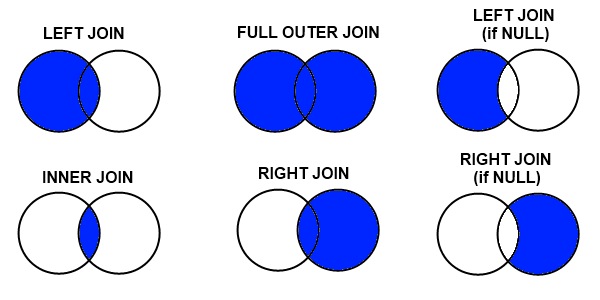
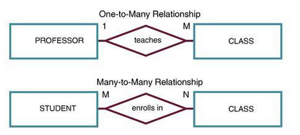
Note that using JOIN introduces potential change in our data context: One to Many and Many to Many relationships.
Troubleshooting JOINs
Make sure that your results are as expected, so consider what the observation is (the row), and rule check other columns:
- is your expected unique column unique?
- Is there duplicate data elsewhere?
A common check to see if your data is not unique is throwing a HAVING clause in your JOIN.
HAVING
Whereas WHERE is used for precomputation, HAVING is a postcomputation clause, filtering the data after the database engine has done the query's work.
SELECT
    t1.c1,
    t1.c2,
    AVG(t2.c2)
FROM t1
INNER JOIN t2 ON t1.c1 = t2.c2
GROUP BY t1.c1, t1.c2
HAVING AVG(t2.c2) > 10;
SELECT
    poll_date,
    AVG(obama_pct)
FROM polls
GROUP BY poll_date
HAVING AVG(obama_pct) > 50;
*pandas*
polls_group = polls.groupby('poll_date').obama_pct.filter(lambda x: x.mean() > 50)
*end_pandas*
Note in this context HAVING allows us to filter on the computed column AVG(t2.c2) after the GROUP BY has run.
Extensibility (Postgres coolness!)
All SQL databases are finetuned to audiences with slightly different functionality. Since we are connecting to a postgres database, we can learn and adopt additional functionality not common in others, like MySQL.
Partitioning, Window Functions
Window functions allow you to subgroup aggregations. Two common needs for this are:
- Providing a comparitive summary of averages or other statistical functions against different group bys;
rank()ing data observations
SELECT
    col1,
    col2,
    rank() over (PARTITION BY col ORDER BY col)
FROM table;
The following:
SELECT
    user_id,
    order_total,
    rank() over (PARTITION BY user_id ORDER BY order_date)
FROM table;
Would create a table that looks like this:
user_id, order_total, rank()
1      , 100        , 1
2      , 80         , 1
1      , 25         , 2
5      , 70         , 1
1      , 120        , 3
Notes:
- rank() is a specific postgres function for ranking and ordering, though any aggregation will do here.
- We can use as many window functions as we'd like.
- Window functions allow us to aggregate in different ways! What would this following SQL query generate?
SELECT
    yearid,
    teamid,
    AVG(salary) over (PARTITION BY yearid, teamid),
    AVG(salary) over (PARTITION BY yearid)
FROM salaries
Questions
- Back to polls! We have a poll_id; how could rank the poll_ids of the top three obama_pct and romney_pct per state?
- We have a table of year, team, games played, and games won. What's the SQL to rank the years for each team based on win percentage?
Subselects (all sql)
There is a lot of additional, great functionality about postgres, like even writing linear regressions:
SELECT
    regr_intercept(yearid, LOG(salary)),
    regr_slope(yearid, LOG(salary)),
    regr_r2(yearid, LOG(salary))
FROM salaries
WHERE salary > 0;
But often SQL has to be "tricked" into thinking the data is not aggregated, particularly with rank(). We'll subselects to explain this:
SELECT col1
FROM (SELECT
    col1,
    col2
    FROM table) table2
In this arbitrary example we can at least see that queries can be nested. We don't see much additional functionality here, but imagine in the orders case:
SELECT *
FROM (SELECT
        user_id,
        order_total,
        rank() over (PARTITION BY user_id ORDER BY order_date) as "order_number"
    FROM table) orders
WHERE order_number = 2
We now get access to the rank in the WHERE (window functions will not work in HAVING due to complexities). You can also join on subselects:
SELECT
    users.platform,
    orders.*
FROM users
INNER JOIN (SELECT
        user_id,
        order_total,
        rank() over (PARTITION BY user_id ORDER BY order_date) as "order_number"
    FROM table) orders on users.id = orders.user_id
WHERE order_number = 2
Connecting via Python
We'll be using a pandas connector alongside SQLAlchemy to connect to this database. Please follow slack for instructions, however the syntax for connecting should be as follows:
from sqlalchemy import create_engine
import pandas as pd
cnx = create_engine('postgresql://username:password@ip_address:port/dbname')
for queries we'll use the pandas syntax:
pd.read_sql_query(query, connection)
The tables we'll need are below. If you need to look at columns, we can use this function:
def show_columns(table, con):
    from pandas import read_sql_table
    return read_sql_table(table, con).columns
Do your best to answer the following questions! They are sorted from simplest to most difficult in terms of SQL execution. If you'd like to practice your pandas syntax, submit both your SQL and pandas code (assuming tables were dataframes).
- Show all playerids and salaries with a salary in the year 1985 above 500k.
- Show the team for each year that had a rank of 1.
- How many schools are in schoolstate of CT?
- How many schools are there in each state?
- What was the total spend on salaries by each team, each year?
- Find all of the salaries of shortstops (fieldings, pos) for the year 2012.
- What is the first and last year played for each player?
- Who has played the most all star games?
- Which school has generated the most distinct players?
- Which school has generated the most expensive players? (expensive defined by their first year's salary).
- Show the 5 most expensive salaries for each team in the year 2014.
- Partition the average salaries by team and year, against year. Find players that were paid more than 1 standard deviation above the average salary for that team and year. Show a count by playerid.
- Calculate the win percentage. convert w and g into numerics (floats) to do so. (
w::numeric, for example) rank()the total spend by team each year against their actual rank that year. Is there a correlation of spend to performance?
Setting up Postgres
This is an incredibly complicated subject matter! Macs should try using homebrew and PCs can use their native installer. Check out their installation guide for more details. If you start reading through and have no idea what they mean, DO NOT attempt to set up postgres on your machine.
Reading / Next Steps
- Read through Hadley Wickham's paper on tidy data. While code samples are written in R it is an incredibly familiar concept and important on how we think about querying.
- Additional comparisons between pandas and sql syntax on the pandas website.
- Some recommended GUIs for interacting with postgres (and other databases):
- If you're looking for something in python between pandas and psycopg2 in terms of complexity, dataset is a great python module to learn, particularly for moving data around.
- Additional SQL Help:
- SQL Bootcamp from GA (MySQL)
- SQLZOO can switch between engines
- w3schools has a practice database.
- SQLSchool