
[PLOTLY'S MATLAB API]
WELCOME! This Notebook is designed to demonstrate the use of the Plotly MATLAB API and to showcase three **\*NEW\*** API functions:
[INITIAL SETUP]
The Plotly MATLAB API has been embedded into our MATLAB toolboxes and our Plotly credentials have been saved using plotlysetup.m. In order to start using the Plotly MATLAB API all we have to do now is start MATLAB! More information regarding installation / setting up the Plotly MATLAB API can be found on the ONLINE DOCUMENTATION.
Throughout this notebook we will be using the super awesome pymatbridge package to communicate with MATLAB from Python. Everything that comes below the %%matlab decorator will now be read as MATLAB code! To use the MATLAB API on your own machine, simply open the MATLAB application as you normally would.
>> OPEN YOUR MATLAB ENVIRONMENT!
%load_ext pymatbridge
Starting MATLAB on ZMQ socket ipc:///tmp/pymatbridge
Send 'exit' command to kill the server
..MATLAB started and connected!
The following code can be used to embed your Plotly plots within your own webpage.
from IPython.display import HTML

def show_plot(url, width=700, height=500):
    s = '<iframe height="%s" id="igraph" scrolling="no" frameborder = 0 seamless="seamless" src="%s" width="%s"></iframe>' %\
    (height, "/".join(map(str,[url, width, height])), width)
    return HTML(s)
[fig2plotly.m]
Plot a MATLAB figure object with Plotly!
>> TELL MATLAB WHERE TO FIND THE EXAMPLE DATA!
%%matlab

api_path = ('/Users/chuckbronson/Documents/PLOTLY/MATLAB_API_REPO/TEST_PLOTS');
addpath(genpath(api_path));
[EXAMPLE 1]
%%matlab
%%%%%%%%%%%%%%%%%%%%%%%%%%%%%%%%%%%%%%%%%%%%%%%%%%%%
% FROM MATLAB PLOT GALLERY %
% http://www.mathworks.com/discovery/gallery.html %
%%%%%%%%%%%%%%%%%%%%%%%%%%%%%%%%%%%%%%%%%%%%%%%%%%%%
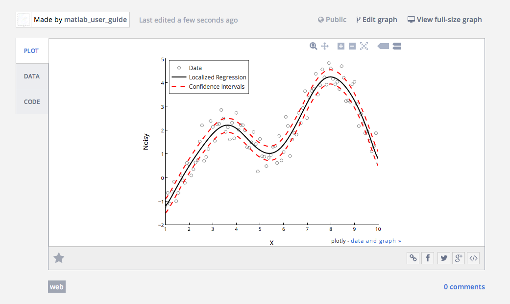
load fitdata x y yfit;
fig = figure;
scatter(x, y, 'k');
line(x, yfit, 'color', 'k', 'linestyle', '-', 'linewidth', 2);
line(x, yfit + 0.3, 'color', 'r', 'linestyle', '--', 'linewidth', 2);
line(x, yfit - 0.3, 'color', 'r', 'linestyle', '--', 'linewidth', 2);
legend('Data', 'Localized Regression', 'Confidence Intervals', 2);
xlabel('X');
ylabel('Noisy');
%%%%%%%%%%%%%%%%%%%%%%%%%%%%%%%
% PLOTLY API CODE %
%%%%%%%%%%%%%%%%%%%%%%%%%%%%%%%
resp = fig2plotly(fig);
The above plot is the ouptut from calling the scatter and line functions inherent in MATLAB. Using the fig2plotly.m function, we are able to extract the relevant data from the MATLAB figure object and throw the output over to Plot.ly! The returned response variable, resp, is a structure array which contains a url field with the address of our plot:
%%matlab
resp.url
ans =

https://plot.ly/~bronsolo/71
Let's have a look at the newly produced line and scatter plot in Plotly!
show_plot('https://plot.ly/~bronsolo/71')
Nice! We can see how the fig2plotly.m function is able to parse all the relevant information for the MATLAB figure object and generate an awesome looking plot, the data for which is now stored on the cloud! This means you'll never have to worry about where your data is saved on your computer and you can share your newly created plot by simply embedding the link within your website or throwing it over to Facebook or Twitter!
Another great thing about Plotly is the interactivity of the graphs. Try scrolling over the newly created plot to view the labelled data. Holding shift while clicking and dragging allows you to pan. Click and drag to zoom and double click to revert back to the original view!
We can also now take advantage of the interactive Web App! You can view/edit all our newly created plots on your online account. By default fig2plotly.m will open your default browser and load your Plotly account to view the newly created plot. All the data associated with the plot has been stored and conveniently formatted in a spreadsheet that can be accessed by clicking on the the "View data" link on the right (below).
By clicking on the "Save & edit" link on the left (above), we are able to access the main web GUI! This will allow us to tweak and experiment with plotting layout and style without having to write lines upon lines of code. Here is a screen shot of the Plotly web app:
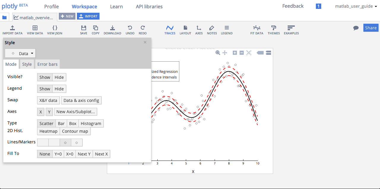
There are also many style/layout themes to choose from and you can even save your own themes to apply to your graphs! Have a go at changing the syle and layout to suite your personal preferences! Here is one that we made:
show_plot('https://plot.ly/~bronsolo/48')
[EXAMPLE 2]
Lets have a look at how fig2plotly.m is able to handle more difficult plot layouts, such as multiple subplots of varying size!
%%matlab

%%%%%%%%%%%%%%%%%%%%%%%%%%%%%%%%%%%%%%%%%%%%%%%%%%%%
%            FROM MATLAB PLOT GALLERY              %
%  http://www.mathworks.com/discovery/gallery.html %
%%%%%%%%%%%%%%%%%%%%%%%%%%%%%%%%%%%%%%%%%%%%%%%%%%%%

fm = 20e3;
fc = 100e3;
tstep = 100e-9;
tmax  = 200e-6;
t = 0:tstep:tmax;
xam = (1 + cos(2*pi*fm*t)).*cos(2*pi*fc*t);
T = 1e-6;
N = 200;
nT = 0:T:N*T;
xn = (1 + cos(2*pi*fm*nT)).*cos(2*pi*fc*nT);
figure;
subplot(2, 2, [1 3]);
plot(nT,xn);
xlabel('t');
ylabel('x[n]');
title('Sampled Every T=1e-6 ');
subplot(2, 2, 2);
plot(t, xam);
axis([0 200e-6 -2 2]);
title('AM Modulated Signal');
subplot(2, 2, 4);
plot(nT, xn);
title('Reconstruction at T=4e-6 ');

%%%%%%%%%%%%%%%%%%%%%%%%%%%%%%%
%        PLOTLY API CODE      %
%%%%%%%%%%%%%%%%%%%%%%%%%%%%%%%
resp = fig2plotly(fig,'strip',1);

show_plot('https://plot.ly/~bronsolo/67/')
Looks Great - fig2plotly.m preserves the subplot layout structure! It also converts the x-axis labels using the concise SI prefix μ = 10-6. You might notice that the colours for the traces generated using fig2plotly.m did not stay blue like the original output from MATLAB. This is because we changed the "strip" property of fig2plotly.m from "false" (default) to "true". In doing so we told fig2plotly.m to change the style used in MATLAB to beautiful default color schemes of Plotly! Go Plotly!
[EXAMPLE 3]
Now let's have a look at some other chart types in MATLAB and apply fig2plotly.m. Let's experiment with bar charts with a double y axis!
%%matlab

%%%%%%%%%%%%%%%%%%%%%%%%%%%%%%%%%%%%%%%%%%%%%%%%%%%%
%            FROM MATLAB PLOT GALLERY              %
%  http://www.mathworks.com/discovery/gallery.html %
%%%%%%%%%%%%%%%%%%%%%%%%%%%%%%%%%%%%%%%%%%%%%%%%%%%%

TBdata = [1990 4889 16.4; 1991 5273 17.4; 1992 5382 17.4; 1993 5173 16.5;
          1994 4860 15.4; 1995 4675 14.7; 1996 4313 13.5; 1997 4059 12.5;
          1998 3855 11.7; 1999 3608 10.8; 2000 3297  9.7; 2001 3332  9.6;
          2002 3169  9.0; 2003 3227  9.0; 2004 2989  8.2; 2005 2903  7.9;
          2006 2779  7.4; 2007 2725  7.2];

years = TBdata(:,1);
cases = TBdata(:,2);
rate  = TBdata(:,3);
fig = figure;
[ax, h1, h2] = plotyy(years, cases, years, rate, 'bar', 'plot');
set(h1, 'FaceColor', [0.8, 0.8, 0.8]);
set(h2, 'LineWidth', 2);
title('Tuberculosis Cases: 1991-2007');
xlabel('Years');
set(get(ax(1), 'Ylabel'), 'String', 'Cases');
set(get(ax(2), 'Ylabel'), 'String', 'Infection rate in cases per thousand');

%%%%%%%%%%%%%%%%%%%%%%%%%%%%%%%
%        PLOTLY API CODE      %
%%%%%%%%%%%%%%%%%%%%%%%%%%%%%%%

filename = 'Tuberculosis Cases';
resp = fig2plotly(fig,'name',filename);

The above plot is the ouptut we receive from calling the plotyy function inherent in MATLAB. Now, Let's grab that url from the resp structure aray and have a look at our newly genereted plot using fig2plotly.m!
%%matlab

resp.url
ans =

https://plot.ly/~bronsolo/82
show_plot('https://plot.ly/~bronsolo/82')
Looks great! Now we can use the Plotly web app to customize style an layout to our personal preference! Alternatively we can use the Plotly declaritive syntax to edit the style and layout with plotly.m, one of the original API functions. To do this, we will need to use another new function that simplifies everything: getplotlyfig.m...
[getplotlyfig.m]
Get data, style, and layout from the plots stored online!
One of Plotly's secret powers is the ability to translate between MATLAB's structure/cell array syntax and JSON! This allows a smooth transition between the your figures in MATLAB and those stored in your Plotly account. In order to grab the data, style, and layout information from your plots living online, we've introduce a new funtion into the API: getplotlyfig.m. In fact, we can go one step further! getploylyfig.m lets you grab the data, style and layout of all Plotly plots as long as they are made public! See a graph you like online? Grab the data, style and layout and make one for yourself!
getplotlyfig.m takes two arguments as input: >> getplotlyfig(file_owner,file_id)
If the provided input arguments are valid, getplotlyfig returns a figure structure with data and layout fields. The data field is a cell array containing the exact same data, and style information as is required for the plotly.m function input. Likewise, the layout structure array contains all the layout information in the same form as is required for the layout field of the optional argument structure array input to plotly.m.
Now that we have a basic understanding of getplotlyfig.m, let's have a go at changing the bar and line colours from our previous example!
%%matlab

%%%%%%%%%%%%%%%%%%%%%%%%%%%%%%%
%       GET PLOTLY FIG!       %
%%%%%%%%%%%%%%%%%%%%%%%%%%%%%%%

plotlyfigure = getplotlyfig('bronsolo','82');

%%%%%%%%%%%%%%%%%%%%%%%%%%%%%%%
%        PLOTLYSTYLE          %
%%%%%%%%%%%%%%%%%%%%%%%%%%%%%%%

% COLOR CHOICES
col1 = '28B78D';
col2 = '#243743';

% BAR CHART STYLE
plotlyfigure.data{1}.marker.color = col1;
plotlyfigure.data{1}.line.width = 2;
plotlyfigure.data{1}.line.color = 'black';
plotlyfigure.data{1}.name = 'Cases';

% LINE STYLE
plotlyfigure.data{2}.line.width = 10;
plotlyfigure.data{2}.line.color = col2;
plotlyfigure.data{2}.name = 'Infection Rate';

% ARGS STRUCTURE
args.filename = 'Tuberculosis Cases';
args.fileopt = 'overwrite';

%%%%%%%%%%%%%%%%%%%%%%%%%%%%%%%
%         PLOTYLAYOUT         %
%%%%%%%%%%%%%%%%%%%%%%%%%%%%%%%

% Y2 AXIS STYLE
plotlyfigure.layout.yaxis2.titlefont.color = col2;
plotlyfigure.layout.yaxis2.tickfont.color = col2;
plotlyfigure.layout.yaxis2.tickcolor = col2;
plotlyfigure.layout.yaxis2.linecolor = col2;
plotlyfigure.layout.yaxis2.linewidth = 5;

% X AXIS STYLE
plotlyfigure.layout.xaxis.mirror = 0;
plotlyfigure.layout.xaxis.showline = 0;
args.layout = plotlyfigure.layout;

resp = plotly(plotlyfigure.data,args)
resp =

         url: 'https://plot.ly/~bronsolo/82'
     message: [1x0 char]
     warning: [1x0 char]
    filename: 'Tuberculosis Cases'
       error: [1x0 char]
show_plot('https://plot.ly/~bronsolo/82')
Awesome! We changed the names of the bar and line data so that when we scroll over the plot we get a nicely labeled interactive output. Give it a try!
[EXAMPLE 4]
[EXAMPLE 5]
Nice, what about contour plots?
%%matlab

%%%%%%%%%%%%%%%%%%%%%%%%%%%%%%%%%%%%%%%%%%%%%%%%%%%%
%            FROM MATLAB PLOT GALLERY              %
%  http://www.mathworks.com/discovery/gallery.html %
%%%%%%%%%%%%%%%%%%%%%%%%%%%%%%%%%%%%%%%%%%%%%%%%%%%%

load mtBruno Longitude Latitude Elevation;
fig = figure;
contour(Longitude, Latitude, Elevation, 8);
title('Mount Bruno Elevation');
xlabel('Longitude');
ylabel('Latitude');


%%%%%%%%%%%%%%%%%%%%%%%%%%%%%%%
%        PLOTLY API CODE      %
%%%%%%%%%%%%%%%%%%%%%%%%%%%%%%%

filename = 'Mount Bruno';
resp = fig2plotly(fig,'strip',1,'name',filename);

Good job MATLAB - now let's look at the Plotly graph we created!
%%matlab

resp.url
ans =

https://plot.ly/~bronsolo/81
show_plot('https://plot.ly/~bronsolo/81/')
So awesome! Now we can add a few more modifications to make this contour plot really pop...
%%matlab

%%%%%%%%%%%%%%%%%%%%%%%%%%%%%%%
%        PLOTLY STYLE         %
%%%%%%%%%%%%%%%%%%%%%%%%%%%%%%%

plotlyfigure = getplotlyfig('bronsolo','81');
plotlyfigure.data{1}.contours.coloring = 'lines';

% ARGS STRUCTURE
args.filename = 'Mount Bruno';
args.fileopt = 'overwrite';

%%%%%%%%%%%%%%%%%%%%%%%%%%%%%%%
%        PLOTLY LAYOUT        %
%%%%%%%%%%%%%%%%%%%%%%%%%%%%%%%
plotlyfigure.layout.colorbar.show = 1;
args.layout = plotlyfigure.layout;

resp = plotly(figure2.data,args);
show_plot('https://plot.ly/~bronsolo/81')
[EXAMPLE 6]
As a last example, let's look at heatmaps! A little audio analysis anyone?
%%matlab

% This is an example of how to add a horizontal colorbar to a plot in MATLAB
%
% Read about the <http://www.mathworks.com/help/matlab/ref/colorbar.html |colorbar|> function in the MATLAB documentation
%
% Go to <http://www.mathworks.com/discovery/gallery.html MATLAB Plot Gallery>
%
% Copyright 2012 The MathWorks, Inc.

% Load spine data
load spine X;

% Create an image plot of the spine data
figure;
imagesc(X);
colormap bone;

resp = fig2plotly(fig);
resp.url
ans =

https://plot.ly/~bronsolo/71

show_plot('https://plot.ly/~bronsolo/71')
So Awesome!
Get data, style, and layout from the plots stored online!
[saveplotlyfig.m]
Save your Plotly figure as an image!
# CSS styling within IPython notebook
from IPython.core.display import HTML
def css_styling():
    styles = open("./css/style_notebook.css", "r").read()
    return HTML(styles)
css_styling()