Test plots for the colormap creator app
In [134]:
%matplotlib inline
Load the script
In [370]:
run color_creator.py
In [7]:
from IPython.html.widgets import interact
1) Lab space cut at a given L level
lightness L lives between 0 and 100. a and b between -128 and +127 (not totally sure), using skimage.color implementation of conversion functions.
In [12]:
plot_ab_plane(25)

In [13]:
plot_ab_plane(50)

In [14]:
plot_ab_plane(75)

Interactive plot of the Lab space cut
In [360]:
%matplotlib inline
In [282]:
interact(plot_ab_plane, L=(0., 100., 2));
TODO (low priority): record an animation of L varying between 0 and 100.
http://matplotlib.org/examples/animation/basic_example_writer.html
Control points in the Lab space
In [581]:
%run color_creator.py
In [582]:
# Blue Green Orange L20-80
pts_lab = [
    (20, 57, -77),
    (40, -9, -25),
    (60, -61, 59),
    (80, 10, 75),
]
plot_lab_pts(pts_lab, markersize=20);
plt.title('Blue Green Orange L20-80');

In [583]:
pts_lab_interp = interp_lab(pts_lab, 5)
pts_lab_interp.shape
Out[583]:
(16, 3)
In [584]:
plot_lab_pts(pts_lab_interp, markersize=10);
plt.title('Blue Green Orange L20-80');

In [585]:
cmap = cmap_from_lab_pts(pts_lab)
cmap(0.0), cmap(1.0)
Out[585]:
((0.077676457080707972, 0.01153735488219438, 0.65379846568805156, 1.0),
 (0.97942192712752985, 0.73967094129870081, 0.16519518694123592, 1.0))
In [586]:
plot_cmap(cmap, title='Blue Green Orange L20-80')
Out[586]:
<matplotlib.axes._subplots.AxesSubplot at 0x7f40470764d0>

In [587]:
plot_cmap(cmap_from_lab_pts(pts_lab, n_interp=5),
          title='Blue Green Orange, with 5 interpolated pts');

For comparison: Brewer's YlGnBu
In [588]:
plot_cmap(mpl.cm.YlGnBu_r, title='YlGnBu (reversed)');

Full demo function:
- colormap
- a-b line plot
- test function colormap
In [589]:
demo_cmap(pts_lab)


Test function for colormap plots
In [590]:
def tfun_3hills(x,y):
    '''2D function on [-1,1]x[-1,1], with 3 hills of different heights,
    and one wide hole
    '''
    def bell(x,y):
        return np.exp(-(x**2+y**2))
    z = 0
    z -= bell(x,y)
    z += bell((x-0.7)*4, y*4)
    z += bell(x*4, (y-0.7)*4)*2
    z += bell((x+0.7)*4, y*4)*3
    return z
In [591]:
x = np.linspace(-1,1, 300)
plt.plot(x, tfun_3hills(x, 0));
plt.title('cut along the x axis, at y=0')
plt.xlabel('x');

In [624]:
pts_lab = np.array(
      [[  5.        ,  30.27572536, -43.70877636],
       [ 28.5       ,  -9.58731303, -19.99279149],
       [ 50.        , -42.63831321,  16.08578122],
       [ 67.5       , -54.49630564,  65.03153721],
       [ 95.        , -17.66083979,  92.27969003]])

cmap = cmap_from_lab_pts(pts_lab)
In [630]:
def plot_tfun(tfun, cmap, reverse=False):
    y,x = np.ogrid[-1:1:100j, -1:1:100j]
    z = tfun(x,y)
    if reverse:
        z = -z
    fig, ax = plt.subplots(1,1, figsize=(5,3), num='cmap test')


    im = ax.imshow(z, origin='lower', cmap=cmap, extent=[-1,1, -1, 1])
    plt.colorbar(im, ax=ax)
    ax.set_title('cmap test')

    fig.tight_layout()

plot_tfun(tfun_3hills, cmap)

In [632]:
plot_tfun(tfun_3hills, cmap, reverse=True)

In [626]:
def plot_tfun_compare(tfun, cmap, reverse=False):
    y,x = np.ogrid[-1:1:100j, -1:1:100j]
    z = tfun(x,y)
    if reverse:
        z = -z
    fig, ax = plt.subplots(2,2, figsize=(10,8))

    cmaps = [[cmap, 'YlGnBu_r'],
             ['gray', 'jet']]

    for i in [0,1]:
        for j in [0,1]:
            im = ax[i,j].imshow(z, origin='lower', cmap=cmaps[i][j], extent=[-1,1, -1, 1]);
            plt.colorbar(im, ax=ax[i,j])
            if i == 0 and j == 0:
                title = 'cmap under test'
            else:
                title='cmap "{}"'.format(cmaps[i][j])
            ax[i,j].set_title(title)

    fig.tight_layout()
In [628]:
plot_tfun_compare(tfun_3hills, cmap)

In [629]:
plot_tfun_compare(tfun_3hills, cmap, reverse=True)

Interactive editor
In [609]:
%matplotlib inline
In [610]:
pts_lab = [
 [ 5., 30,-43],
 [ 28.5, -5,-20],
 [ 50.,-42, 18],
 [ 67.5,-68, 67],
 [ 95., -18, 91]]

demo_cmap(pts_lab, 'Blue Green Yellow L5-95')


In [633]:
%matplotlib qt
ed = LabEditor(pts_lab)
# before moving the points
ed.pts_lab
Out[633]:
array([[  5.        ,  30.27572536, -43.70877636],
       [ 28.5       ,  -9.58731303, -19.99279149],
       [ 50.        , -42.63831321,  16.08578122],
       [ 67.5       , -54.49630564,  65.03153721],
       [ 95.        , -17.66083979,  92.27969003]])
Screenshot of the point editor.
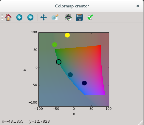
The available sRGB gamut is displayed for the point being moved (circled in black). This gamut heavily depends on L value.
In [617]:
# after moving the points:
ed.pts_lab
Out[617]:
array([[  5.        ,  28.76193909, -41.18579924],
       [ 28.5       ,  51.97332853,   0.44332312],
       [ 50.        ,  75.18471797,  42.82933862],
       [ 67.5       ,  35.57397729,  73.10506398],
       [ 95.        , -17.40854208,  89.50441521]])
In [618]:
%matplotlib inline
demo_cmap(ed.pts_lab, title='cmap, after editing')


Gallery of colormaps
a) Blue → Green → Yellow family
In [508]:
# Blue Green Orange
pts_lab = [
    (20, 57, -77),
    (40, -9, -25),
    (60, -61, 59),
    (80, 10, 75),
]
demo_cmap(pts_lab, 'Blue Green Orange L20-80')

In [509]:
# Blue Green  Yellow
pts_lab = [
 [ 10., 40,-52],
 [ 30., -5,-20],
 [ 50.,-42, 18],
 [ 70.,-68, 67],
 [ 90., -9, 87]]
demo_cmap(pts_lab, 'Blue Green Yellow L10-90')


In [510]:
# Blue Green  Yellow L10-90, after adjustment
pts_lab = np.array([[ 10.        ,  36.41129032, -49.87903226],
       [ 30.        ,   0.84677419, -29.55645161],
       [ 50.        , -31.33064516,   3.46774194],
       [ 70.        , -31.33064516,  52.58064516],
       [ 90.        ,  -8.46774194,  88.99193548]])
demo_cmap(pts_lab, 'Blue Green Yellow L10-90, curved')


In [511]:
# Blue Green  Yellow L5-95, after a weird adjustment
pts_lab = np.array([[  5.        ,  20.32258065, -10.08064516],
       [ 28.5       ,  11.00806452, -37.17741935],
       [ 50.        , -33.87096774,   6.00806452],
       [ 67.5       ,  17.78225806,  60.2016129 ],
       [ 95.        , -20.32258065,  92.37903226]])
demo_cmap(pts_lab, 'Blue Green Yellow L5-95, snake')


b) Blue → Magenta → Yellow family
In [519]:
%run color_creator.py
In [520]:
# Blue Magenta Orange
pts_lab = np.array(
      [[ 20.        ,  56.73387097, -76.12903226],
       [ 50.        ,  77.90322581,  11.08870968],
       [ 80.        ,  11.00806452,  79.67741935]])
demo_cmap(pts_lab, 'Blue Magenta Orange L20-80')


→ Nice looking, but notice that the interpolated purple points are saturated!
In [521]:
# Blue Magenta Yellow
pts_lab = [
 [ 10., 36, -49],
 [ 30., 56, -24],
 [ 50., 77, 4],
 [ 70., 38, 45],
 [ 90.,  -9, 87]]
demo_cmap(pts_lab, 'Blue Magenta Yellow L10-90')


In [522]:
# Blue Magenta Yellow, after tuning
pts_lab = np.array([[ 10.        ,  30.48387097, -43.10483871],
       [ 30.        ,  55.88709677, -13.46774194],
       [ 50.        ,  74.51612903,  30.56451613],
       [ 70.        ,  34.71774194,  60.2016129 ],
       [ 90.        ,  -9.31451613,  79.67741935]])
demo_cmap(pts_lab, 'Purple Red Yellow L10-90')


In [619]:
# Blue Magenta Yellow, L5-95
pts_lab = np.array([[  5.        ,  28.76193909, -41.18579924],
       [ 28.5       ,  51.97332853,   0.44332312],
       [ 50.        ,  75.18471797,  42.82933862],
       [ 67.5       ,  35.57397729,  73.10506398],
       [ 95.        , -17.40854208,  89.50441521]])
demo_cmap(pts_lab, 'Purple Red Yellow L5-95')
