Getting started with into
- Full tutorial available at http://github.com/ContinuumIO/blaze-tutorial
- Install software with
conda install -c blaze blaze
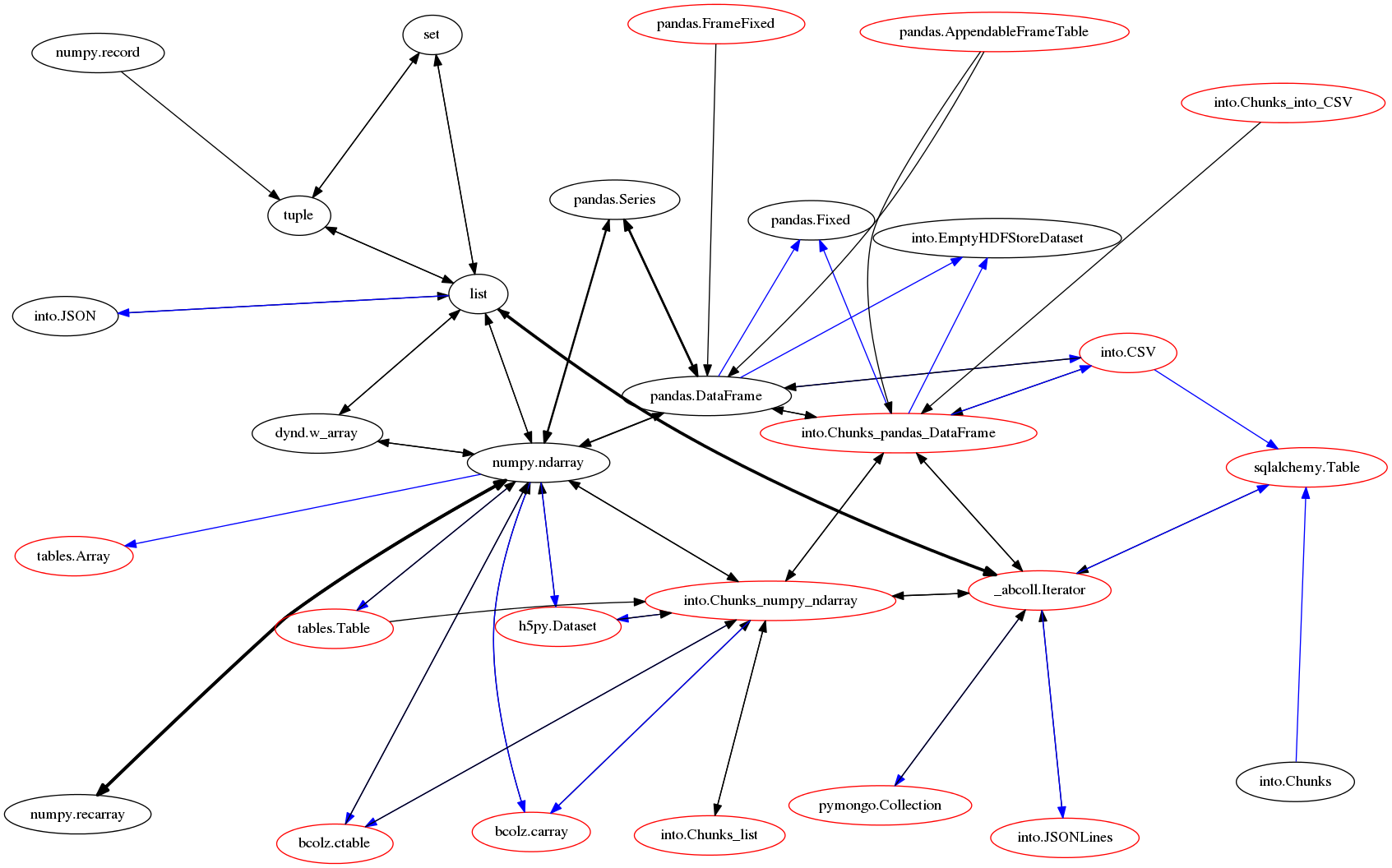
Nodes represent data formats. Arrows represent functions that migrate data from one format to another. Red nodes are possibly larger than memory.
This differs from most data migration systems, which always migrate data through a common format.
This common strategy is simpler in design and easier to get right, so why does into use a more complex design?
Some edges are very fast
For example transforming an np.ndarray to a pd.Series or a list to Iterator only requires us to manipulate metadata which can be done quickly; the bytes of data remain untouched. In many cases transfering data through a common format can be much slower.
For example consider CSV -> SQL migration. Using Python iterators as a common central format we're bound by SQLAlchemy's insertion code which maxes out at around 2000 records per second. Using CSV loaders native to the database (e.g. PostgreSQL Copy) we achieve more than 50000 records per second, turning an overnight task into 20 minutes.
Efficient data migration is intrinsically messy in practice. The into graph reflects this mess.
How does into use this graph?
When you convert one dataset into another, Into walks the graph above and finds the minimum path. Each edge corresponds to a single function and that edge is weighted according to relative cost. E.g. if we transform a CSV file into a set we can see the stages through which our data moves.
from into import into, convert, append, CSV
path =  convert.path(CSV, set)

for source, target, func in path:
    print '%25s -> %-25s   via   %s()' % (source.__name__, target.__name__, func.__name__)
                      CSV -> Chunks_pandas_DataFrame     via   CSV_to_chunks_of_dataframes()
  Chunks_pandas_DataFrame -> Iterator                    via   numpy_chunks_to_iterator()
                 Iterator -> list                        via   iterator_to_list()
                     list -> set                         via   iterable_to_set()
Chunks of in-memory data
The red nodes in our graph represent data that might be larger than memory. We we migrate between two red nodes we restrict ourselves to the subgraph of only red nodes so that we never blow up.
Yet we still want to use NumPy and Pandas in these migrations (they're very helpful intermediaries) so we partition our data into a sequence of chunks such that each chunks fit in memory. We describe this data with parametrized types like chunks(np.ndarray) or chunks(pd.DataFrame).
into = convert + append
Recall the two modes of into
# Given type:  Convert source to new object
into(list, (1, 2, 3))
[1, 2, 3]
# Given object: Append source to that object
L = [1, 2, 3]
into(L, (4, 5, 6))
L
[1, 2, 3, 4, 5, 6]
These two modes are actually separate functions, convert and append. Into uses both depending on the situation. A single into call may engage both functions.
You should use into by default, it does some other checks. For the sake of being explicit however, here are examples using convert and append directly.
from into import convert, append

convert(list, (1, 2, 3))
[1, 2, 3]
L = [1, 2, 3]
append(L, (4, 5, 6))
[1, 2, 3, 4, 5, 6]
How to extend into
When we encounter new data formats we may wish to connect them to the into graph. We do this by implementing new versions of discover, convert, and append (if we support appending).
We register new implementations of an operation like convert by creating a new Python function and decorating it with types and a cost.
Example
Here we define how to convert from a DataFrame to a NumPy array
import numpy as np
import pandas as pd

#                 target type, source data, cost
@convert.register(np.ndarray, pd.DataFrame, cost=1.0)
def dataframe_to_numpy(df, **kwargs):
    return df.to_records(index=False)