Optimal Control and Parameter Identification of Dynamcal Systems with Direct Collocation and SymPy
Jason K. Moore
July 8, 2015
SciPy 2015, Austin, Texas, USA

|
|
|
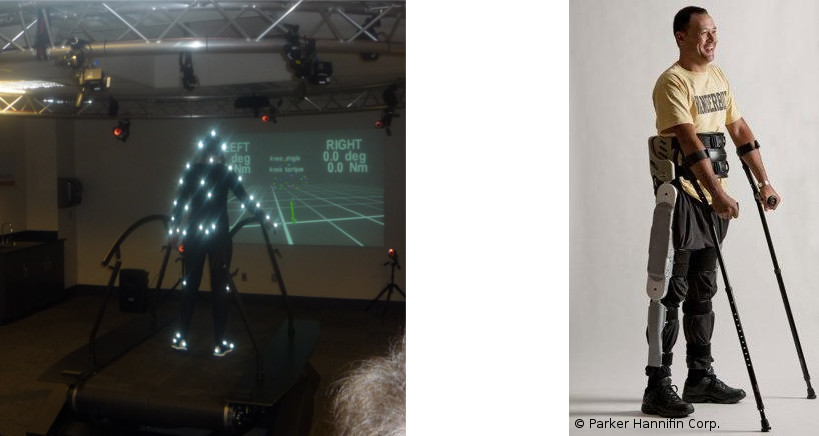
Motivation: Identification of Gait Control
Previous Use Cases: Optimal Gait on Earth, Moon, Mars
Ackermann, M. and van den Bogert, A. J. Predictive simulation of gait at low gravity reveals skipping as the preferred
locomotion strategy. Journal of Biomechanics, 45, 2012
|
Earth: g=9.8 m/s-2 |
Moon: g=1.6 m/s-2 |
Trajectory Optimization Example

1-DoF, 1 parameter pendulum equations of motion
$\dot{\mathbf{x}} = \begin{bmatrix} \dot{\theta}(t) \\ \dot{\omega}(t) \end{bmatrix} = \begin{bmatrix} \omega(t) \\ \frac{g}{l} \sin{\theta}(t) + \mathbf{T} \end{bmatrix}$
Objective: Minimize "effort" and bound the states at
$J(\mathbf{T}) = \min\limits_{\mathbf{T}} \int_{t_0}^{t_f} \mathbf{T}^2 dt$
Boundary conditions
- $\mathbf{\theta}(t_0) = 0$
- $\mathbf{\theta}(t_f) = \pi$
Pendulum figure: https://commons.wikimedia.org/wiki/File:Pendulum_gravity.svg, Creative Commons Attribution-Share Alike 3.0 Unported
Parameter Identification
Find the parameters $\mathbf{p}$ such that the difference between the model simulation, $\mathbf{y}$, and measurements, $\mathbf{y}_m$ is minimized.
Dynamic system
- Equations of Motion: $\dot{\mathbf{x}} = \mathbf{f}(\mathbf{x}, \mathbf{p})$
- Measurement variables: $\mathbf{y} = \mathbf{g}(\mathbf{x}, \mathbf{p})$
Objective
$$\min\limits_\mathbf{p} J(\mathbf{p})$$where $$J(\mathbf{p}) = \int [\mathbf{y}_m - \mathbf{y}(\mathbf{p})]^2 dt$$
Optimal Control By Shooting
- Repeated simulations are computationally costly (i.e. stiff systems are especially slow)
- Maybe limited to parameterized functions (e.g. polynomials, piecewise constants)
- Too many free variables
- Systems may be unstable and thus have an ill-defined objective
- Local minima are inevitable
- May requires a superb guess
- May need time intensive global optimization methods
Local Minima Example: Simple pendulum
Vyasarayani, Chandrika P., Thomas Uchida, Ashwin Carvalho, and John McPhee.
"Parameter Identification in Dynamic Systems Using the Homotopy Optimization Approach". Multibody System Dynamics 26, no. 4 (2011): 411-24.

1-DoF, 1 parameter pendulum equations of motion
$\dot{\mathbf{x}} = \begin{bmatrix} \dot{\theta}(t) \\ \dot{\omega}(t) \end{bmatrix} = \begin{bmatrix} \omega(t) \\ -p \sin{\theta}(t) \end{bmatrix}$
Objective: Minimize least squares
$J(p) = \min\limits_{p} \int_{t_0}^{t_f} [\theta_m(t) - \theta(\mathbf{x}, p, t)]^2 dt$
Direct Collocation
Benefits
- Fast computation times
- Handles unstable systems with ease
- Less susceptible to local minima
Disadvantages
- Accurate solution requires large number of nodes
- Memory management for large sparse matrices and operations
- Tedious and error prone to form gradients, Jacobians, and Hessians
Our Direct Collocation Implementation
Implicit Continous Equations of Motion
No need to solve for $\dot{\mathbf{x}}$.
$$\mathbf{f}(\dot{\mathbf{x}}, \mathbf{x}, \mathbf{r}, \mathbf{p}, t) = 0$$- $\mathbf{x}, \dot{\mathbf{x}}$: states and their derivatives
- $\mathbf{r}$: exogenous inputs
- $\mathbf{p}$: constant parameters
Discretization
First order discrete integration options:
Backward Euler:
$\mathbf{f}(\frac{\mathbf{x}_i - \mathbf{x}_{i-1}}{h} , \mathbf{x}_i, \mathbf{r}_i, \mathbf{p}, t_i) = 0$
Midpoint Rule:
$\mathbf{f}(\frac{\mathbf{x}_{i + 1} - \mathbf{x}_i}{h}, \frac{\mathbf{x}_i + \mathbf{x}_{i + 1}}{2}, \frac{\mathbf{r}_i + \mathbf{r}_{i + 1}}{2}, \mathbf{p}, t_i) = 0$
Nonlinear Programming Formulation
$$\min\limits_{\theta} J(\theta)$$$$\textrm{where } \mathbf{\theta} = [\mathbf{x}_i, \dots, \mathbf{x}_N, \mathbf{r}_i, \ldots, \mathbf{r}_N, \mathbf{p}]$$$$\textrm{subject to } \mathbf{f}(\mathbf{x}_i, \mathbf{x}_{i+1}, \mathbf{r}_i, \mathbf{r}_{i+1}, \mathbf{p}, t_i) = 0 \textrm{ and } \theta_L \leq \theta \leq \theta_U$$Software Tool: opty
http://github.com/csu-hmc/opty
- User specifies continous symbolic:
- objective
- equations of motion (explicit or implicit)
- additional constraints
- bounds on free variables: $\mathbf{x}, \mathbf{r}, \mathbf{p}$
- EoMs can be generated with PyDy (http://pydy.org)
- Effficient just-in-time compiled C code is generated for functions that evaluate:
- objective and its gradient
- constraints and its Jacobian
- NLP problem automatically formed for IPOPT
- Open source: BSD license
- Written in Python
Example Code: Specify Equations of Motion
$$\dot{\mathbf{x}} = \begin{bmatrix} \dot{\theta}(t) \\ \dot{\omega}(t) \end{bmatrix} = \begin{bmatrix} \omega(t) \\ -p \sin{\theta}(t) + T(t) \end{bmatrix}$$
Symbolic EoM
# Specify symbols for the parameters
p, t = symbols('p, t')

# Specify the functions of time
theta, omega, theta_m, T = symbols('theta, omega, theta_m, T', cls=Function)

# Specify the symbolic equations of motion
eom = Matrix([theta(t), omega(t)]).diff(t) - Matrix([omega(t), -p * sin(theta(t) + T(t))])
Discretization
# Choose discretization values
num_nodes = 1000
interval = 0.01  # seconds
Example Code: Trajectory Optimization
Objective
obj = Integral(T(t)**2, t)
Boundary Contraints
boundary_constraints = (theta(0.0), theta(duration) - pi / 2, omega(0.0), omega(duration))
Define Problem
prob = Problem(obj,  # symbolic objective
               eom,  # symbolic equations of motion
               (theta(t), omega(t)),  # system symbolic states
               num_nodes,
               interval,
               known_parameter_map={p: 9.81},
               instance_constraints=boundary_constraints)
Example Code: Solve
# Set an initial guess
initial_guess = random(prob.num_free)

# Solve the system
solution, info = prob.solve(initial_guess)
The Problem Class: Objective
- Converts objective integral to discrete form
- Computes analytic gradient of objective wrt to discrete variables
- Generates efficient NumPy functions for objective and gradient
*Still in development
The Problem Class: Constraints
- Converts continous EoM to discrete versions
- Computes the analytic Jacobian wrt to discrete variables
- Generates efficient C code to "ufuncify" discrete EoM and Jacobian evaluations
- Generates Cython wrapper for C code
- Compiles Cython wrapper
- NumPy functions are generated for instance constraints
The Problem Class: Solve
- IPOPT data structure is formed with cyipopt
- Bounds on variables are set
- IPOPT settings are set
- Solve is called!

Case Study: Minamal Effort Double Pendulum Swing Up
<img src="two-link-pendulum-with-cart.svg"style="float:right;margin=5px;" width=400px/>
- Two-link pendulum with lateral force applied to base
- States: $\mathbf{x}=[q_0 \quad q_1 \quad q_2 \quad u_0 \quad u_1 \quad u_2]^T$
- Unknown exogoneous input: $\mathbf{F}$
- Known parameters: $[m_0, m_1, m_2, l_0, l_1]$
- Boundary conditions:
- $q_0(t_0)=0$
- $q_1(t_0),q_1(t_0)=-\frac{\pi}{2}$
- $q_1(t_f),q_1(t_f)=\frac{\pi}{2}$
- $u_0(t_0), u_2(t_0), u_2(t_0), u_0(t_f), u_1(t_f), u_2(t_f)=0$
Trajectory Opimization Problem Specification
Given the boundary conditions can we find the optimal input trajectory such that the "effort" is minimized?
$$\min\limits_\theta J(\mathbf{\theta}), \quad J(\mathbf{\theta})= \sum_{i=1}^N h [\mathbf{T}_i]^2$$where
$$ \mathbf{\theta} = [\mathbf{x}_1, \ldots, \mathbf{x}_N, \mathbf{T}_i, \ldots \mathbf{T}_N] $$Subject to the constraints:
$$\mathbf{f}(\mathbf{x}_i, \mathbf{T}_i)=0, \quad i=1 \ldots N$$And the initial guess:
$$\mathbf{\theta}_0 = [\mathbf{0}]$$For, $N$ = 500:
- 24008 free variables
- Jacobian matrix with 38933 non-zero entries
Demo

Case Study: Human Control Parameter Identification
Plant

- Torque driven two-link inverted pendulum with an accelerating base.
- States: $\mathbf{x}=[\theta_a \quad \theta_h \quad \omega_a \quad \omega_h]^T$
- Exogoneous inputs:
- Controlled: $\mathbf{r}_c = [T_a \quad T_h]^T$
- Specified: $\mathbf{r}_k = [a]$
- Known parameters: $\mathbf{p}_k$
Open Loop Equations of Motion
$$\dot{\mathbf{x}} = \mathbf{f}_o(\mathbf{x}, \mathbf{r}_c, \mathbf{r}_k, \mathbf{p}_k, t)$$
Lumped Passive+Active Controller
- True human controller is practically impossible to isolate and identify
- Identify a controller for a similar system that causes the same behavior as the real system
Simple State Feedback
$$\mathbf{r}_c(t) = -\mathbf{K}\mathbf{x}(t)$$Unknown Parameters
$$\mathbf{p}_u = \mathrm{vec}(\mathbf{K})$$Closed Loop Equations of Motion
$$\dot{\mathbf{x}} = \mathbf{f}_c(\mathbf{x}, \mathbf{r}_k, \mathbf{p}_k, \mathbf{p}_u, t)$$Generate Data
Specify the psuedo-random platform acceleration
$$a(t)=\sum_{i=1}^{12} A_i\sin(\omega_i t) \quad \mathrm{where,} \quad 0.15 \mathrm{rad/s} < \omega_i < 15.0 \mathrm{rad/s}$$Choose a stable controller
$$ \mathbf{K} = \begin{bmatrix} 950 & 175 & 185 & 50 \\ 45 & 290 & 60 & 26 \end{bmatrix} $$Generate Data
Simulate closed loop system under the influence of perturbations for 60 seconds, sampled at 100 Hz
$$ \dot{\mathbf{x}} = \mathbf{f}_c(\mathbf{x}, \mathbf{r}_k, \mathbf{p}_k, \mathbf{p}_u, t) $$Add Gaussian measurement noise
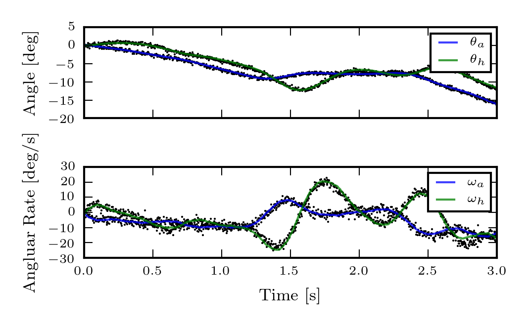
$$\mathbf{x}_m(t) = \mathbf{x}(t) + \mathbf{v}_x(t) \\ a_m(t) = a(t) + v_a(t)$$- $\sigma_\theta$ = 0.3 deg
- $\sigma_\omega$ = 4 deg/s
- $\sigma_a$ = 0.42 ms-2
Parameter Identification Problem Specification
Given noisy measurements of the states, $\mathbf{x}_m$, and the platform acceleration, $a_m$, can we identify the controller parameters $\mathbf{K}$?
$$\min\limits_\theta J(\mathbf{\theta}), \quad J(\mathbf{\theta})= \sum_{i=1}^N h [\mathbf{x}_{mi} - \mathbf{x}_i]^2$$where
$$ \mathbf{\theta} = [\mathbf{x}_1, \ldots, \mathbf{x}_N, \mathbf{p}_u] $$Subject to the constraints:
$$\mathbf{f}_{ci}(\mathbf{x}_i, a_{mi}, \mathbf{p}_u)=0, \quad i=1 \ldots N$$And the initial guess:
$$\mathbf{\theta}_0 = [\mathbf{x}_{m1}, \ldots, \mathbf{x}_{mN}, \mathbf{0}]$$For, $N$ = 6000:
- 24008 free variables
- 23996 x 24008 Jacobian matrix with 384000 non-zero entries
Demo
Results
Converges in 11 iterations in 2.8 seconds of computation time.
| Known | Identified | Error | |
|---|---|---|---|
| $k_{00}$ | 950 | 946 | -0.4% |
| $k_{01}$ | 175 | 177 | 1.4% |
| $k_{02}$ | 185 | 185 | -0.2% |
| $k_{03}$ | 50 | 55 | 9.4% |
| $k_{10}$ | 45 | 45 | 1.1% |
| $k_{11}$ | 290 | 289 | -0.3% |
| $k_{12}$ | 60 | 59 | -2.1% |
| $k_{13}$ | 26 | 27 | 4.2% |
Identified State Trajectories
Conclusion
- Direct collocation is suitable for biomechanical parameter identification and trajectory optimization
- Computation speeds are orders of magnitude faster than shooting
- Parameter identification accuracy improves with # nodes
- Complex problems can be solved with few lines of code and high level mathematical abstractions
Questions?
- Social media: moorepants
- Personal website: http://moorepants.info
- SymPy: http://sympy.org
- PyDy: http://pydy.org
- opty: http://github.com/csu-hmc/opty
- Human Motion and Control Lab: http://hmc.csuohio.edu