In this Notebook, we learn how to add interactivity to graphs using matplotlib widgets. A widget (phonetic: ˈwɪdʒɪt') is an interactive part of a user interface. Examples are radio buttons, where you can select only one button at a time, check buttons, where you can select multiple buttons at a time, and sliders which you can, well, slide to change something in the graph.
%pylab qt
Populating the interactive namespace from numpy and matplotlib
Creating a widget
The process for creating a widget is the same for each widget:
- Create a figure with the desired graph and make sure the components of the graph that you want to change are stored as objects
- Add a new axis to a graph for the widget.
- Create the widget and add it to the appropriate axis.
- Write a function that is called when the state of the widget is changed (i.e., a radio button is selected or the slider is moved).
- Tell the widget to call this function when its state is changed.
- When all is done, call
show()
Widgets need to be imported from the matplotlib.widgets package. All widgets are listed here. In this Notebook, we will use radio buttons and sliders.
Radio buttons
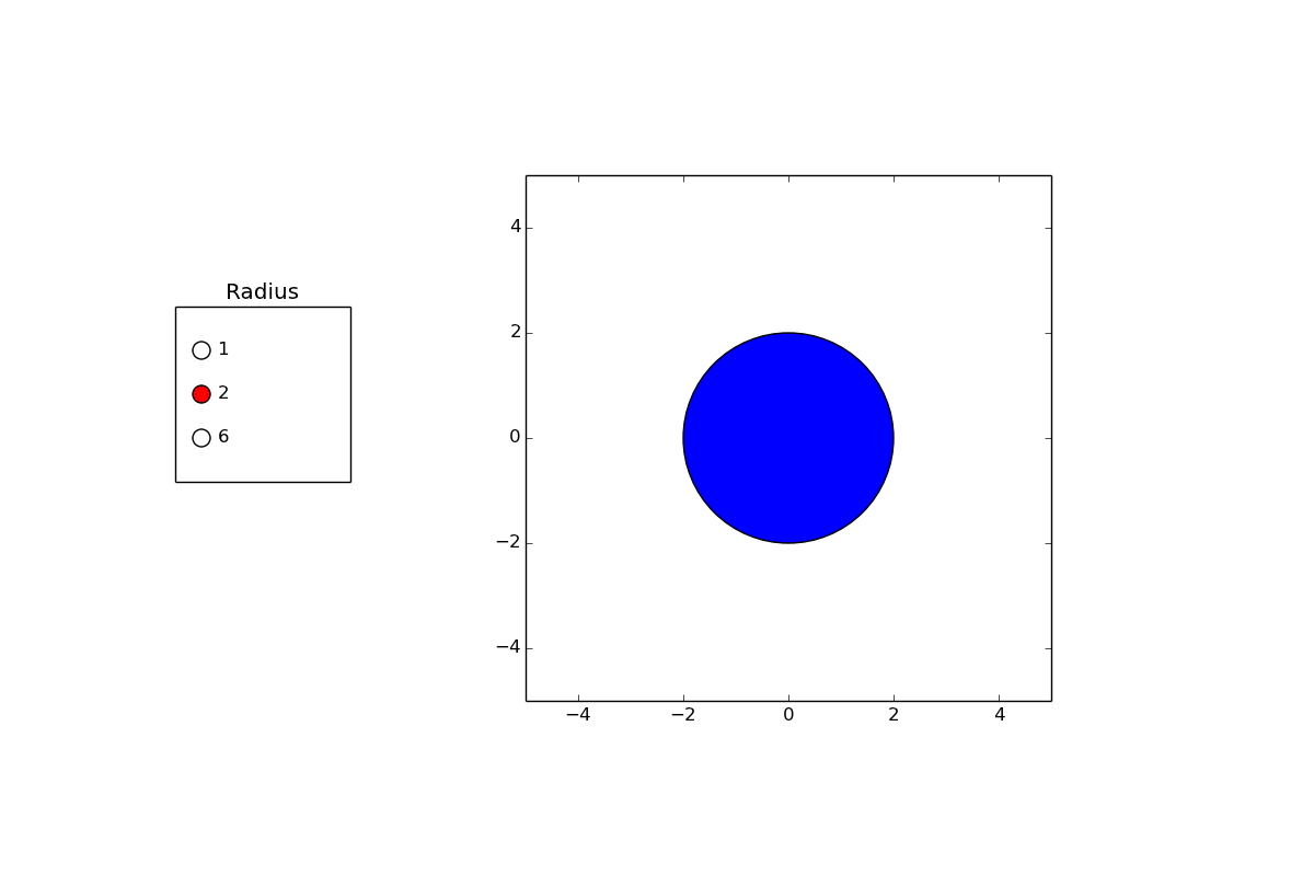
Consider the graph of a circle. We will add radio buttons to change the radius of the circle. The code and an image of the interactive window are shown below.
In step 1 we create a figure, add an an axis, and add a circle to the axis. The circle object is stored as c1. The axis is created with the axes command, and the aspect ratio is set with the keyword argument aspect='equal' so that a circle looks like a circle and not an ellipse. Finally, the data limits of the axes are set. This is important as matplotlib won't do that for you when you add a patch.
In step 2 we create a second axis that will contain the radio buttons; the axis is called rax. The aspect ratio is again set to 'equal' so that the buttons look like cirles (rather than ellipses), and the title of the axis is set to Radius.
In step 3 a RadioButtons object is created and called radio. The RadioButtons class takes two arguments: the axis to which the radio buttons are added (here it is rax), and a list with the labels of the buttons. We create three buttons with labels 1, 2, and 6. The labels need to be given as a list of strings. Two additional keyword arguments are provided: active=1 tells the RadioButtons class that upon creation button number 1 is active (the first button is number zero) as the circle has a radius $R=2$ when we create it. The keyword argument activecolor='r' tells the RadioButtons class to use the color red for the active button.
In step 4 the function setradius is defined (we can choose whatever name we find appropriate). The function takes one argument, which is the label of one of the radio buttons. When the function is called, it sets the radius of circle c1 to the value of the label of the radio button. Note that the label of the radio button is a string, so we have to convert it to a float first. The function ends by calling the draw() function that redraws the figure with a circle with the new radius.
In step 5, the radio object is told that when one of the radio buttons is clicked it should call the setradius function. The on_clicked function is part of the RadioButtons class.
Finally, in step 6 we call show() to show the figure.
When you run the code below, a seperate figure window is created in which you can change the radius of the circle interactively by clicking on the radio buttons. A still image of what you will see is shown below the code.
from pylab import *
from matplotlib.widgets import RadioButtons
from matplotlib.patches import Circle
# step 1
fig = figure(figsize=(12,8))
ax1 = fig.add_axes([0.4,0.1,0.4,0.8], aspect='equal')
c1 = Circle(xy=(0,0),radius=2)
ax1.add_patch(c1)
ax1.set_xlim(-5,5)
ax1.set_ylim(-5,5)
# step 2
rax = fig.add_axes([0.1,0.45,0.2,0.2], aspect='equal', title='Radius')
# step 3
radio = RadioButtons( rax, ['1','2','6'], active=1, activecolor='r')
# step 4
def setradius(label):
    c1.set_radius(float(label))
    draw()
# step 5
radio.on_clicked(setradius)
# step 6
show()
Execise 1. Radio buttons to set color
Add a second set of radio buttons to change the color of the circle shown in the previous example. You may want to relocate the radio buttons that set the radius of the circle to a more convenient place on the graph. Provide at least three options for setting the color of the circle. Note that a Circle object has a set_color function.
Changing the shape of a line
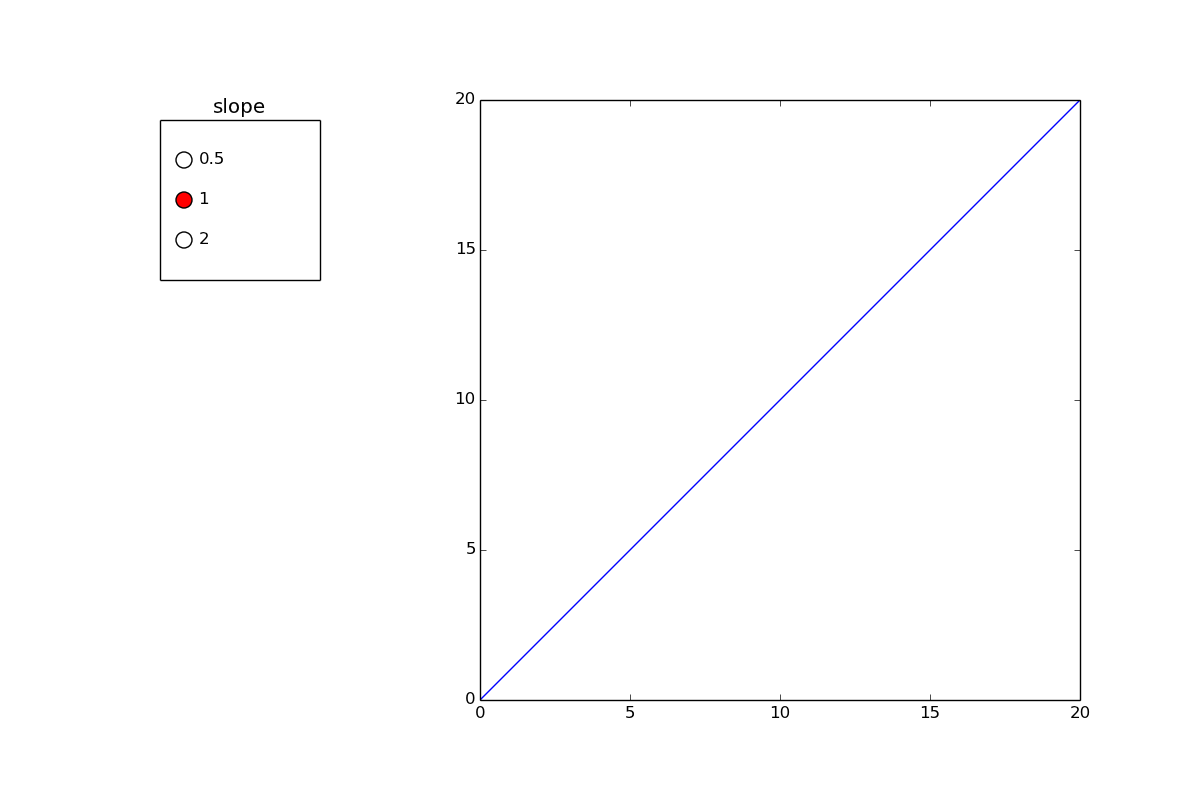
Adding a line is similar to adding a circle. A line is added as a Line2D object. In the example below, we create a straight line $y=ax+b$. A Line2D object is created and added to the axis and the limits of the axes are set. Then we add radio buttons to change the slope of the line. A still image of the interactive window is shown below the code.
from pylab import *
from matplotlib.widgets import RadioButtons
from matplotlib.lines import Line2D

# Step 1: Create figure with the line
fig = figure(figsize=(12,8))
ax = fig.add_axes([0.4,0.1,0.5,0.8],aspect='equal')
a = 1
b = 0
x = linspace(0,20,10)
y = a * x + b
line1 = Line2D(x,y)
ax.add_line(line1)
xlim(0,20)
ylim(0,20)

# Radio buttons for slope
ax1 = fig.add_axes([0.1,0.65,0.2,0.2], aspect='equal', title='slope') # step 2
slope = RadioButtons( ax1, ['0.5','1','2'], active=1, activecolor='r') # step 3
def setslope(label): # step 4
    a = float(label)
    y = a * x + b
    line1.set_ydata(y)
    draw()
slope.on_clicked(setslope)  # step 5

show()  # step 6
In the function setslope the slope is set to the value selected with the radio buttons. But, since the slope a is set inside a function, it is not set outside the function. After all, any variable created inside a function only exists inside the function and not outside. But in this case, we want to change the slope a outside the function as well. For that we define the variable a to be global inside the setslope function. We also add a second set of radio buttons to set the $y$-intercept b, where b is defined as global inside the setintercept function.
from pylab import *
from matplotlib.widgets import RadioButtons
from matplotlib.lines import Line2D

# Create figure with line
fig = figure(figsize=(12,8))
ax = fig.add_axes([0.4,0.1,0.5,0.8],aspect='equal')
a = 1
b = 0
x = linspace(0,20,10)
y = a * x + b
line1 = Line2D(x,y)
ax.add_line(line1)
xlim(0,20)
ylim(0,20)

# Radio buttons for slope and intercept
ax1 = fig.add_axes([0.1,0.65,0.2,0.2], aspect='equal', title='slope') # step 2
ax2 = fig.add_axes([0.1,0.25,0.2,0.2], aspect='equal')
slope = RadioButtons( ax1, ['0.5','1','2'], active=1, activecolor='r') # step 3
intercept = RadioButtons( ax2, ['0','5','10'], active=0, activecolor='r')
def setslope(label): # step 4
    global a
    a = float(label)
    y = a * x + b
    line1.set_ydata(y)
    draw()
def setintercept(label):
    global b
    b = float(label)
    y = a * x + b
    line1.set_ydata(y)
    draw()
slope.on_clicked(setslope)  # step 5
intercept.on_clicked(setintercept)

show()  # step 6
Exercise 2. Deflection of a beam
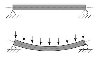
Consider the elastic deflection of a beam with a uniform load $q$. The beam is supported by two simple supports (see figure below). The formula for the shape $y(x)$ of the deformed beam is
$y = -\frac{qx}{24EI} (L^3 - 2Lx^2 + x^3)$
where $E$ is the elasticity modulus, $I$ is the area moment of intertia, and $L$ is the length of the beam. Make a graph using $q=100$ N/mm, $L=5000$ mm, $I= 1067\cdot 10^6$ mm$^4$ (i.e., a beam of width 200 mm and height 400 mm), and the elasticity modulus of wood $E=11000$ N/mm$^2$. Set the $x$-limits of the graph from $0$ to $5000$, and the $y$-limits of the graph from $-100$ to $0$ (you won't see anything if you forget to set the limits, as they are not updated automatically in the OO modus). Add two sets of radiobuttons. In the first set of radiobuttons, the type of material can be selected: wood ($E=11000$ N/mm$^2$), concrete ($E=35000$ N/mm$^2$), or aluminum ($E=71000$ N/mm$^2$). In the second set of radiobuttons the load can be selected: $50$, $100$ or $200$ N/mm. Make sure that once a radiobutton is selected, the shape of the deflected beam changes accordingly.
Slider
Consider again the graph of a circle but now with an initially horizontal line through the center of the circle. We will add a slider to the graph that allows the user to rotate the circle from -180$^\circ$ to +180$^\circ$. The proces consists again of the six steps defined at the top of this Notebook. In step 1 we create the graph. The line is added as a Line2D class called line1 and has only two points. The first point is $(x,y)=(-R\cos(\alpha),-R\sin(\alpha))$, the second point is $(x,y)=(R\cos(\alpha),R\sin(\alpha))$; initially the angle is $\alpha=0$ and the radius is $R=3$. In step 2 we create the axis to which we will add the slider. In step 3 we create the slider and call it angleslider. The Slider class takes four input arguments: the axis to add the slider to, the name that is printed next to the slider, the minimum value and the maximum value. There are also a number of keyword arguments (use Slider? after you import it). We use one here: we set the initial value of the slider to zero using the valinit keyword. In step 4 we define an update function setangle that will be called when the value of the slider is changed. It takes as argument the value of the slider, it changes the $x$ and $y$ data of the line, and it draws the updated figure. In step 5 we tell the slider to call the setangle function when the value is changed using the on_changed function. And finally in step 6 we show the figure. A still image of a more complicated version of this figure is shown below Exercise 4.
from pylab import *
from matplotlib.widgets import Slider
from matplotlib.patches import Circle

# Step 1: Create figure with circle and line
fig = figure(figsize=(6,8))
ax1 = fig.add_axes([0.1,0.3,0.8,0.6], aspect='equal')
R = 3
c1 = Circle(xy=(0,0),radius=R,fc='violet')
ax1.add_patch(c1)
angle = 0
line1 = Line2D(xdata = [-R*cos(angle),R*cos(angle)],\
            ydata = [-R*sin(angle),R*sin(angle)],color='k')
ax1.add_line(line1)
xlim(-5,5)
ylim(-5,5)
# Step 2: Create axis for slider
axslider = fig.add_axes([0.2,0.15,0.6,0.05])
# Step 3: Create slider and add to axis
angleslider = Slider(axslider, 'Angle', -180, 180, valinit=0)
# Step 4: Function to call when slider is changed
def setangle(val):
    angle = val * pi/180
    line1.set_xdata([-R*cos(angle),R*cos(angle)])
    line1.set_ydata([-R*sin(angle),R*sin(angle)])
    draw()
# Step 5: Tell the angleslider what function to call when its value has changed
angleslider.on_changed(setangle)
# Step 6: Call show()
show()
Exercise 3. Sliders
Part 1 Add a small blue circle with radius 0.2 at the intersection of the line and circle (see figure below but without the second slider). Initially, when $\alpha=0$, the center of the small circle is at $(x,y)=(R,0)$. Make sure that the small circle rotates with the line when the angle is changed with the slider.
Part 2
Add a second slider to the graph you created for Part 1. The second slider allows the user to change the radius of the circle between 2 and 4. Note that you have to create a second slider axis under step 2, a second slider under step 3, a second update function under step 4, and you need to tell the new slider which function to call when it is changed under step 5. The current setangle function uses the variable R as the radius of the large circle. In this new implementation, the radius is set by the new slider. The current value of a slider is stored in the val attribute of the slider. Hence, if your slider is called slidername, then slidername.val is the current value of the slider. When you write your code, it is important that you first define both sliders under step 3, as the update functions you define in step 4 need to have access to the value of the other slider (either the radius or the angle). When you are done, you graph should look something like the figure below (and the sliders should work, or course).

Answers to the exercises
from pylab import *
from matplotlib.widgets import RadioButtons
from matplotlib.patches import Circle

# Create figure with circle
fig = figure(figsize=(12,8))
ax1 = fig.add_axes([0.4,0.1,0.5,0.8], aspect='equal')
c1 = Circle(xy=(0,0),radius=2,color='blue')
ax1.add_patch(c1)
xlim(-5,5)
ylim(-5,5)

# Radio buttons for radius of circle
rax = axes([0.1,0.65,0.2,0.2], aspect='equal', title='Radius')
radio = RadioButtons( rax, ['1','2','6'], active=1, activecolor='r')
def setradius(label):
    c1.set_radius(float(label))
    draw()
radio.on_clicked(setradius)

# Radio buttons for color of circle
cax = axes([0.1,0.25,0.2,0.2], aspect='equal', title='Color')
color = RadioButtons( cax, ['violet','blue','green','black'], active=1, activecolor='r')
def setcolor(label):
    c1.set_color(label)
    draw()
color.on_clicked(setcolor)

show()
from pylab import *
from matplotlib.widgets import RadioButtons
from matplotlib.lines import Line2D

fig = figure()
ax1 = fig.add_axes([0.1,0.4,0.8,0.5])
E = 11e3
I = 1067e6
q = 100
L = 5000
x = linspace(0,L,100)
d = -q * x / (24*E*I) * (L**3 - 2*L*x**2 + x**3)
line = Line2D(xdata=x,ydata=d)
ax1.add_line(line)
xlabel('x (mm)')
ylabel('deflection (mm)')
xlim(0,L)
ylim(-100,0)

ax2 = fig.add_axes([0.05,0.05,0.2,0.2],aspect='equal',title='material')
ax3 = fig.add_axes([0.55,0.05,0.2,0.2],aspect='equal',title='qload')

Emod = RadioButtons( ax2, ['wood','concrete','aluminum'], active=0, activecolor='r')
qload = RadioButtons( ax3, ['50','100','200'], active=1, activecolor='r')
def setEmod(label):
    global E
    if label == 'wood': E = 11e3
    if label == 'concrete': E = 35e3
    if label == 'aluminum': E = 71e3
    d = -q * x / (24*E*I) * (L**3 - 2*L*x**2 + x**3)
    line.set_ydata(d)
    draw()
def setqload(label):
    global q
    q = float(label)
    d = -q * x / (24*E*I) * (L**3 - 2*L*x**2 + x**3)
    line.set_ydata(d)
    draw()
Emod.on_clicked(setEmod)
qload.on_clicked(setqload)

show()
from pylab import *
from matplotlib.widgets import Slider
from matplotlib.patches import Circle

fig = figure(figsize=(6,8))
ax1 = fig.add_axes([0.1,0.3,0.8,0.6], aspect='equal')
R = 3
c1 = Circle(xy=(0,0),radius=R,fc='violet')
ax1.add_patch(c1)
angle = 0
l1 = Line2D(xdata = [-R*cos(angle),R*cos(angle)],\
            ydata = [-R*sin(angle),R*sin(angle)],color='k')
ax1.add_line(l1)
c2 = Circle(xy=(R*cos(angle),R*sin(angle)),radius=0.2,fc='b')
ax1.add_patch(c2)
xlim(-5,5)
ylim(-5,5)

axslider = fig.add_axes([0.2,0.15,0.6,0.05])
angleslider = Slider(axslider, 'Angle', -180, 180, valinit=0)
axslider2 = fig.add_axes([0.2,0.05,0.6,0.05])
angleslider2 = Slider(axslider2, 'Radius', 2, 4, valinit=3)

def update(val):
    angle = val * pi/180
    R = angleslider2.val
    l1.set_xdata([-R*cos(angle),R*cos(angle)])
    l1.set_ydata([-R*sin(angle),R*sin(angle)])
    c2.center = R*cos(angle),R*sin(angle)
    draw()

def update2(R):
    angle = angleslider.val * pi/180
    l1.set_xdata([-R*cos(angle),R*cos(angle)])
    l1.set_ydata([-R*sin(angle),R*sin(angle)])
    c2.center = R*cos(angle),R*sin(angle)
    c1.radius = R
    draw()

angleslider.on_changed(update)
angleslider2.on_changed(update2)

show()