Notebook 2: Arrays
In this notebook, we will do math on arrays using functions of the numpy package. A nice overview of numpy functionality can be found here. We will also make plots. We start by telling the Jupyter Notebooks to put all graphs inline. Then we import the numpy package and call it np, and we import the plotting part of the matplotlib package and call it plt. We will add these three lines at the top of all upcoming notebooks as we will always be using numpy and matplotlib.
%matplotlib inline
import numpy as np
import matplotlib.pyplot as plt
One-dimensional arrays
There are many ways to create arrays. For example, you can enter the individual elements of an array
np.array([1, 7, 2, 12])
array([ 1, 7, 2, 12])
Note that the array function takes one sequence of points between square brackets.
Another function to create an array is np.ones(shape), which creates an array of the specified shape filled with the value 1.
There is an analogous function np.zeros(shape) to create an array filled with the value 0 (which can also be achieved with 0 * np.ones(shape)). Next to the already mentioned np.linspace function there is the np.arange(start, end, step)
function, which creates an array starting at start, taking steps equal to step and stopping before it reaches end. If you don't specify the step,
it is set equal to 1. If you only specify one input value, it returns a sequence starting at 0 and incrementing by 1 until the specified value is reached (but again, it stops before it reaches that value)
print(np.arange(1, 7)) # Takes default steps of 1 and doesn't include 7
print(np.arange(5)) # Starts at 0 end ends at 4, giving 5 numbers
[1 2 3 4 5 6]
[0 1 2 3 4]
Recall that comments in Python are preceded by a #.
Arrays have a dimension. So far we have only used one-dimensional arrays.
Hence the dimension is 1.
For one-dimensional arrays, you can also compute the length (which is part of Python and not numpy), which returns the number of values in the array
x = np.array([1, 7, 2, 12])
print('number of dimensions of x:', np.ndim(x))
print('length of x:', len(x))
number of dimensions of x: 1
length of x: 4
The individual elements of an array can be accessed with their index. Indices start at 0. This may require a bit of getting used to. It means that the first value in the array has index 0. The index of an array is specified using square brackets.
x = np.arange(20, 30)
print('array x:', x)
print('value with index 0:', x[0])
print('value with index 5:', x[5])
array x: [20 21 22 23 24 25 26 27 28 29]
value with index 0: 20
value with index 5: 25
A range of indices may be specified using the colon syntax:
x[start:end_before] or x[start:end_before:step]. If the start isn't specified, 0 will be used. If the step isn't specified, 1 will be used.
x = np.arange(20, 30)
print(x)
print(x[0:5])
print(x[:5])  # same as previous one
print(x[3:7])
print(x[2:9:2])  # step is 2
[20 21 22 23 24 25 26 27 28 29]
[20 21 22 23 24]
[20 21 22 23 24]
[23 24 25 26]
[22 24 26 28]
You can also start at the end and count back. Generally, the index of the end is not known. You can find out how long the array is and access the last value by typing x[len(x) - 1] but it would be inconvenient to have to type len(arrayname) all the time. Luckily, there is a shortcut: x[-1] is the same as x[len(x) - 1] and represents the last value in the array. For example:
xvalues = np.arange(0, 100, 10)
print(xvalues)
print(xvalues[len(xvalues) - 1])  # last value in array
print(xvalues[-1])  # much shorter
print(xvalues[-1::-1])  # start at the end and go back with steps of -1
[ 0 10 20 30 40 50 60 70 80 90]
90
90
[90 80 70 60 50 40 30 20 10  0]
You can assign one value to a range of an array by specifying a range of indices,
or you can assign an array to a range of another array, as long as the ranges have the same length. In the last example below, the first 5 values of x (specified as x[0:5]) are given the values [40, 42, 44, 46, 48].
x = 20 * np.ones(10)
print(x)
x[0:5] = 40
print(x)
x[0:5] = np.arange(40, 50, 2)
print(x)
[20. 20. 20. 20. 20. 20. 20. 20. 20. 20.]
[40. 40. 40. 40. 40. 20. 20. 20. 20. 20.]
[40. 42. 44. 46. 48. 20. 20. 20. 20. 20.]
Exercise 1, Arrays and indices
Create an array of zeros with length 20. Change the first 5 values to 10. Change the next 10 values to a sequence starting at 12 and increasig with steps of 2 to 30 (do this with one command). Set the final 5 values to 30. Plot the value of the array on the $y$-axis vs. the index of the array on the $x$-axis. Draw vertical dashed lines at $x=4$ and $x=14$ (i.e., the section between the dashed lines is where the line increases from 10 to 30). Set the minimum and maximum values of the $y$-axis to 8 and 32 using the ylim command.
Arrays, Lists, and Tuples
A one-dimensional array is a sequence of values that you can do math on. Next to an array, Python has several other data types that can store a sequence of values. The first one is called a list and is entered between square brackets. The second one is a tuple (you are right, strange name), and it is entered with parentheses. The difference is that you can change the values in a list after you create them, and you can not do that with a tuple. Other than that, for now you just need to remember that they exist, and that you cannot do math with either lists or tuples. When you do 2 * alist, where alist is a list, you don't multiply all values in alist with the number 2. What happens is that you create a new list that contains alist twice (so it adds them back to back). The same holds for tuples. That can be very useful, but not when your intent is to multiply all values by 2. In the example below, the first value in a list is modified. Try to modify one of the values in btuple below and you will see that you get an error message:
alist = [1, 2, 3]
print('alist', alist)
btuple = (10, 20, 30)
print('btuple', btuple)
alist[0] = 7  # Since alist is a list, you can change values
print('modified alist', alist)
#btuple[0] = 100  # Will give an error
#print(2 * alist)
alist [1, 2, 3]
btuple (10, 20, 30)
modified alist [7, 2, 3]
Lists and tuples are versatile data types in Python. We already used lists without realizing it when we created our first array with the command np.array([1, 7, 2, 12]). What we did is we gave the array function one input argument: the list [1, 7, 2, 12], and the array function returned a one-dimensional array with those values. Lists and tuples can consist of a sequences of pretty much anything, not just numbers. In the example given below, alist contains 5 things: the integer 1, the float 20.0, the word python, an array with the values 1,2,3, and finally, the function len. The latter means that alist[4] is actually the function len. That function can be called to determine the length of an array as shown below. The latter may be a bit confusing, but it is cool behavior if you take the time to think about it.
alist = [1, 20.0, 'python', np.array([1,2,3]), len]
print(alist)
print(alist[0])
print(alist[2])
print(alist[4](alist[3]))  # same as len(np.array([1,2,3]))
[1, 20.0, 'python', array([1, 2, 3]), <built-in function len>]
1
python
3
Two-dimensional arrays
Arrays may have arbitrary dimensions (as long as they fit in your computer's memory). We will make frequent use of two-dimensional arrays. They can be created with any of the aforementioned functions by specifying the number of rows and columns of the array. Note that the number of rows and columns must be a tuple (so they need to be between parentheses), as the functions expect only one input argument for the shape of the array, which may be either one number or a tuple of multiple numbers.
x = np.ones((3, 4)) # An array with 3 rows and 4 columns
print(x)
[[1. 1. 1. 1.]
 [1. 1. 1. 1.]
 [1. 1. 1. 1.]]
Arrays may also be defined by specifying all the values in the array. The array function gets passed one list consisting of separate lists for each row of the array. In the example below, the rows are entered on different lines. That may make it easier to enter the array, but it is not required. You can change the size of an array to any shape using the reshape function as long as the total number of entries doesn't change.
x = np.array([[4, 2, 3, 2],
              [2, 4, 3, 1],
              [0, 4, 1, 3]])
print(x)
print(np.reshape(x, (2, 6)))  # 2 rows, 6 columns
print(np.reshape(x, (1, 12)))  # 1 row, 12 columns
[[4 2 3 2]
 [2 4 3 1]
 [0 4 1 3]]
[[4 2 3 2 2 4]
 [3 1 0 4 1 3]]
[[4 2 3 2 2 4 3 1 0 4 1 3]]
The index of a two-dimensional array is specified with two values, first the row index, then the column index.
x = np.zeros((3, 8))
x[0, 0] = 100
x[1, 4:] = 200  # Row with index 1, columns starting with 4 to the end
x[2, -1:4:-1] = 400  # Row with index 2, columns counting back from the end with steps of 1 and stop before reaching index 4
print(x)
[[100.   0.   0.   0.   0.   0.   0.   0.]
 [  0.   0.   0.   0. 200. 200. 200. 200.]
 [  0.   0.   0.   0.   0. 400. 400. 400.]]
Arrays are not matrices
Now that we talk about the rows and columns of an array, the math-oriented reader may think that arrays are matrices, or that one-dimensional arrays are vectors. It is crucial to understand that arrays are not vectors or matrices. The multiplication and division of two arrays is term by term
a = np.arange(4, 20, 4)
b = np.array([2, 2, 4, 4])
print('array a:', a)
print('array b:', b)
print('a * b  :', a * b)  # term by term multiplication
print('a / b  :', a / b)  # term by term division
array a: [ 4  8 12 16]
array b: [2 2 4 4]
a * b  : [ 8 16 48 64]
a / b  : [2. 4. 3. 4.]
Exercise 2, Two-dimensional array indices
For the array x shown below, write code to print:
- the first row of
x - the first column of
x - the third row of
x - the last two columns of
x - the 2 by 2 block of values in the upper right-hand corner of
x - the 2 by 2 block of values at the center of
x
x = np.array([[4, 2, 3, 2], [2, 4, 3, 1], [2, 4, 1, 3], [4, 1, 2, 3]])
Visualizing two-dimensional arrays
Two-dimensonal arrays can be visualized with the plt.matshow function. In the example below, the array is very small (only 4 by 4), but it illustrates the general principle. A colorbar is added as a legend. The ticks in the colorbar are specified to be 2, 4, 6, and 8. Note that the first row of the array (with index 0), is plotted at the top, which corresponds to the location of the first row in the array.
x = np.array([[8, 4, 6, 2],
              [4, 8, 6, 2],
              [4, 8, 2, 6],
              [8, 2, 4, 6]])
plt.matshow(x)
plt.colorbar(ticks=[2, 4, 6, 8], shrink=0.8)
print(x)
[[8 4 6 2]
 [4 8 6 2]
 [4 8 2 6]
 [8 2 4 6]]

The colors that are used are defined in the default color map (it is called viridis), which maps the highest value to yellow, the lowest value to purple and the numbers in between varying between blue and green. An explanation of the advantages of viridis can be seen here. If you want other colors, you can choose one of the other color maps with the cmap keyword argument. To find out all the available color maps, go
here. For example, setting the color map to rainbow gives
plt.matshow(x, cmap='rainbow')
plt.colorbar(ticks=np.arange(2, 9, 2), shrink=0.8);

Exercise 3, Create and visualize an array
Create an array of size 10 by 10. Set the upper left-hand quadrant of the array should to 4, the upper right-hand quadrant to 3, the lower right-hand quadrant t0 2 and the lower left-hand quadrant to 1. First create an array of 10 by 10 using the zeros command, then fill each quadrant by specifying the correct index ranges. Visualize the array using matshow. It should give a red, yellow, light blue and dark blue box (clock-wise starting from upper left) when you use the jet colormap.
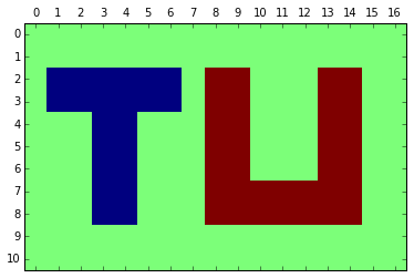
Exercise 4, Create and visualize a slightly fancier array
Consider the image shown below, which roughly shows the letters TU. You are asked to create an array that represents the same TU. First create a zeros array of 11 rows and 17 columns. Give the background value 0, the letter T value -1, and the letter U value +1. Use the jet colormap.
Using conditions on arrays
If you have a variable, you can check whether its value is smaller or larger than a certain other value. This is called a conditional statement. For example:
a = 4
print('a < 2:', a < 2)
print('a > 2:', a > 2)
a < 2: False
a > 2: True
The statement a < 2 returns a variable of type boolean, which means it can either be True or False. Besides smaller than or larger than, there are several other conditions you can use:
a = 4
print('the value of a is', a)
print('a < 4: ', a < 4)
print('a <= 4:', a <= 4) # a is smaller than or equal to 4
print('a == 4:', a == 4) # a is equal to 4. Note that there are 2 equal signs
print('a >= 4:', a >= 4)
print('a > 4: ', a > 4)
print('a != 4:', a != 4) # a is not equal to 4
the value of a is 4
a < 4:  False
a <= 4: True
a == 4: True
a >= 4: True
a > 4:  False
a != 4: False
It is important to understand the difference between one equal sign like a = 4 and two equal signs like a == 4. One equal sign means assignment. Whatever is on the right side of the equal sign is assigned to what is on the left side of the equal sign. Two equal signs is a comparison and results in either True (when both sides are equal) or False.
print(4 == 4)
a = 4 == 5
print(a)
print(type(a))
True
False
<class 'bool'>
You can also perform comparison statements on arrays, and it will return an array of booleans (True and False values) for each value in the array. For example let's create an array and find out what values of the array are below 3:
data = np.arange(5)
print(data)
print(data < 3)
[0 1 2 3 4]
[ True  True  True False False]
The statement data < 3 returns an array of type boolean that has the same length as the array data and for each item in the array it is either True or False. The cool thing is that this array of True and False values can be used to specify the indices of an array:
a = np.arange(5)
print(a)
print(a[[True, True, False, False, True]])
[0 1 2 3 4]
[0 1 4]
When the indices of an array are specified with a boolean array, only the values of the array where the boolean array is True are selected. This is a very powerful feature. For example, all values of an array that are less than, for example, 3 may be obtained by specifying a condition as the indices.
a = np.arange(5)
print('the total array:', a)
print('values less than 3:', a[a < 3])
the total array: [0 1 2 3 4]
values less than 3: [0 1 2]
If we want to replace all values that are less than 3 by, for example, the value 10, use the following short syntax:
a = np.arange(5)
print(a)
a[a < 3] = 10
print(a)
[0 1 2 3 4]
[10 10 10  3  4]
Exercise 5, Replace high and low values in an array
Create an array for variable $x$ consisting of 100 values from 0 to 20. Compute $y=\sin(x)$ and plot $y$ vs. $x$ with a blue line. Next, replace all values of $y$ that are larger than 0.5 by 0.5, and all values that are smaller than $-$0.75 by $-$0.75, and plot the modified $y$ values vs. $x$ using a red line on the same graph.
Exercise 6, Change marker color based on data value
Create an array for variable $x$ consisting of 100 points from 0 to 20 and compute $y=\sin(x)$. Plot a blue dot for every $y$ that is larger than zero, and a red dot otherwise
Select indices based on multiple conditions
Multiple conditions can be given as well. When two conditions both have to be true, use the & symbol. When at least one of the conditions needs to be true, use the '|' symbol (that is the vertical bar). For example, let's plot $y=\sin(x)$ and plot blue markers when $y>0.7$ or $y<-0.5$ (using one plot statement), and a red marker when $-0.5\le y\le 0.7$. Note that when there are multiple conditions, they need to be between parentheses.
x = np.linspace(0, 6 * np.pi, 50)
y = np.sin(x)
plt.plot(x[(y > 0.7) | (y < -0.5)], y[(y > 0.7) | (y < -0.5)], 'bo')
plt.plot(x[(y > -0.5) & (y < 0.7)], y[(y > -0.5) & (y < 0.7)], 'ro');

Exercise 7, Multiple conditions
The file xypoints.dat contains 1000 randomly chosen $x,y$ locations of points; both $x$ and $y$ vary between -10 and 10. Load the data using loadtxt, and store the first row of the array in an array called x and the second row in an array called y. First, plot a red dot for all points. On the same graph, plot a blue dot for all $x,y$ points where $x<-2$ and $-5\le y \le 0$. Finally, plot a green dot for any point that lies in the circle with center $(x_c,y_c)=(5,0)$ and with radius $R=5$. Hint: it may be useful to compute a new array for the radial distance $r$ between any point and the center of the circle using the formula $r=\sqrt{(x-x_c)^2+(y-y_c)^2}$. Use the plt.axis('equal') command to make sure the scales along the two axes are equal and the circular area looks like a circle.
Exercise 8, Fix the error
In the code below, it is meant to give the last 5 values of the array x the values [50, 52, 54, 56, 58] and print the result to the screen, but there are some errors in the code. Remove the comment markers and run the code to see the error message. Then fix the code and run it again.
#x = np.ones(10)
#x[5:] = np.arange(50, 62, 1)
#print(x)
Answers to the exercises
x = np.zeros(20)
x[:5] = 10
x[5:15] = np.arange(12, 31, 2)
x[15:] = 30
plt.plot(x)
plt.plot([4, 4], [8, 32],'k--')
plt.plot([14, 14], [8, 32],'k--')
plt.ylim(8, 32);

x = np.array([[4, 2, 3, 2],
              [2, 4, 3, 1],
              [2, 4, 1, 3],
              [4, 1, 2, 3]])
print('the first row of x')
print(x[0])
print('the first column of x')
print(x[:, 0])
print('the third row of x')
print(x[2])
print('the last two columns of x')
print(x[:, -2:])
print('the four values in the upper right hand corner')
print(x[:2, 2:])
print('the four values at the center of x')
print(x[1:3, 1:3])
the first row of x
[4 2 3 2]
the first column of x
[4 2 2 4]
the third row of x
[2 4 1 3]
the last two columns of x
[[3 2]
 [3 1]
 [1 3]
 [2 3]]
the four values in the upper right hand corner
[[3 2]
 [3 1]]
the four values at the center of x
[[4 3]
 [4 1]]
x = np.zeros((10, 10))
x[:5, :5] = 4
x[:5, 5:] = 3
x[5:, 5:] = 2
x[5:, :5] = 1
print(x)
plt.matshow(x, cmap='jet')
plt.colorbar(ticks=[1, 2, 3, 4], shrink=0.8);
[[4. 4. 4. 4. 4. 3. 3. 3. 3. 3.]
 [4. 4. 4. 4. 4. 3. 3. 3. 3. 3.]
 [4. 4. 4. 4. 4. 3. 3. 3. 3. 3.]
 [4. 4. 4. 4. 4. 3. 3. 3. 3. 3.]
 [4. 4. 4. 4. 4. 3. 3. 3. 3. 3.]
 [1. 1. 1. 1. 1. 2. 2. 2. 2. 2.]
 [1. 1. 1. 1. 1. 2. 2. 2. 2. 2.]
 [1. 1. 1. 1. 1. 2. 2. 2. 2. 2.]
 [1. 1. 1. 1. 1. 2. 2. 2. 2. 2.]
 [1. 1. 1. 1. 1. 2. 2. 2. 2. 2.]]

x = np.zeros((11, 17))
x[2:4, 1:7] = -1
x[2:9, 3:5] = -1
x[2:9, 8:10] = 1
x[2:9, 13:15] = 1
x[7:9, 10:13] = 1
print(x)
plt.matshow(x, cmap='jet')
plt.yticks(range(11, -1, -1))
plt.xticks(range(0, 17));
plt.ylim(10.5, -0.5)
plt.xlim(-0.5, 16.5);
[[ 0.  0.  0.  0.  0.  0.  0.  0.  0.  0.  0.  0.  0.  0.  0.  0.  0.]
 [ 0.  0.  0.  0.  0.  0.  0.  0.  0.  0.  0.  0.  0.  0.  0.  0.  0.]
 [ 0. -1. -1. -1. -1. -1. -1.  0.  1.  1.  0.  0.  0.  1.  1.  0.  0.]
 [ 0. -1. -1. -1. -1. -1. -1.  0.  1.  1.  0.  0.  0.  1.  1.  0.  0.]
 [ 0.  0.  0. -1. -1.  0.  0.  0.  1.  1.  0.  0.  0.  1.  1.  0.  0.]
 [ 0.  0.  0. -1. -1.  0.  0.  0.  1.  1.  0.  0.  0.  1.  1.  0.  0.]
 [ 0.  0.  0. -1. -1.  0.  0.  0.  1.  1.  0.  0.  0.  1.  1.  0.  0.]
 [ 0.  0.  0. -1. -1.  0.  0.  0.  1.  1.  1.  1.  1.  1.  1.  0.  0.]
 [ 0.  0.  0. -1. -1.  0.  0.  0.  1.  1.  1.  1.  1.  1.  1.  0.  0.]
 [ 0.  0.  0.  0.  0.  0.  0.  0.  0.  0.  0.  0.  0.  0.  0.  0.  0.]
 [ 0.  0.  0.  0.  0.  0.  0.  0.  0.  0.  0.  0.  0.  0.  0.  0.  0.]]

x = np.linspace(0, 20, 100)
y = np.sin(x)
plt.plot(x, y, 'b')
y[y > 0.5] = 0.5
y[y < -0.75] = -0.75
plt.plot(x, y, 'r');

x = np.linspace(0, 20, 100)
y = np.sin(x)
plt.plot(x[y > 0], y[y > 0], 'bo')
plt.plot(x[y <= 0], y[y <= 0], 'ro');

x, y = np.loadtxt('xypoints.dat')
plt.plot(x, y, 'ro')
plt.plot(x[(x < -2) & (y >= -5) & (y < 0)], y[(x < -2) & (y >= -5) & (y < 0)], 'bo')
r = np.sqrt((x - 5) ** 2 + y ** 2)
plt.plot(x[r < 5], y[r < 5], 'go')
plt.axis('scaled');

x = np.ones(10)
x[5:] = np.arange(50, 60, 2)
print(x)
[ 1. 1. 1. 1. 1. 50. 52. 54. 56. 58.]