NetCDF is a set of software libraries and self-describing, machine-independent data formats that support the creation, access, and sharing of array-oriented scientific data.
Structure of the netCDF file
netcdf air.sig995.1950 {
dimensions:
    lon = 144 ;
    lat = 73 ;
    time = UNLIMITED ; // (365 currently)
variables:
float lat(lat) ;
	lat:units = "degrees_north" ;
	lat:actual_range = 90.f, -90.f ;
	lat:long_name = "Latitude" ;
	lat:standard_name = "latitude" ;
	lat:axis = "Y" ;
float lon(lon) ;
	lon:units = "degrees_east" ;
	lon:long_name = "Longitude" ;
	lon:actual_range = 0.f, 357.5f ;
	lon:standard_name = "longitude" ;
	lon:axis = "X" ;
double time(time) ;
	time:long_name = "Time" ;
	time:delta_t = "0000-00-01 00:00:00" ;
	time:avg_period = "0000-00-01 00:00:00" ;
	time:standard_name = "time" ;
	time:axis = "T" ;
	time:units = "hours since 1800-01-01 00:00:0.0" ;
	time:actual_range = 1314864., 1323600. ;
float air(time, lat, lon) ;
	air:long_name = "mean Daily Air temperature at sigma level 995" ;
	air:units = "degK" ;
	air:precision = 2s ;
	air:least_significant_digit = 1s ;
	air:GRIB_id = 11s ;
	air:GRIB_name = "TMP" ;
	air:var_desc = "Air temperature" ;
	air:dataset = "NCEP Reanalysis Daily Averages" ;
	air:level_desc = "Surface" ;
	air:statistic = "Mean" ;
	air:parent_stat = "Individual Obs" ;
	air:missing_value = -9.96921e+36f ;
	air:actual_range = 188.53f, 314.9f ;
	air:valid_range = 185.16f, 331.16f ;

// global attributes:
	:Conventions = "COARDS" ;
	:title = "mean daily NMC reanalysis (1950)" ;
	:description = "Data is from NMC initialized reanalysis\n",
		"(4x/day).  These are the 0.9950 sigma level values." ;
	:platform = "Model" ;
	:references = "http://www.esrl.noaa.gov/psd/data/gridded/data.ncep.reanalysis.html" ;
	:history = "created 99/06/07 by Hoop (netCDF2.3)\n",
		"Converted to chunked, deflated non-packed NetCDF4 2014/09" ;
}
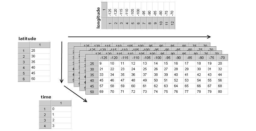
Dimensions
A dimension may be used to represent a real physical dimension, for example, time, latitude, longitude, or height. A dimension might also be used to index other quantities, for example station or model-run-number.
 source: http://trac.osgeo.org/gdal/wiki/ADAGUC
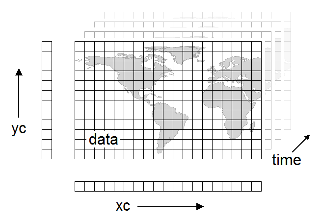
Variables
Variables are used to store the bulk of the data in a netCDF dataset. A variable represents an array of values of the same type. A scalar value is treated as a 0-dimensional array. A variable has a name, a data type, and a shape described by its list of dimensions specified when the variable is created. A variable may also have associated attributes, which may be added, deleted or changed after the variable is created.
 source: http://www.narccap.ucar.edu/users/user-meeting-08/handout/handout.html
Attributes
NetCDF attributes are used to store data about the data (ancillary data or metadata), similar in many ways to the information stored in data dictionaries and schema in conventional database systems. Most attributes provide information about a specific variable. These are identified by the name (or ID) of that variable, together with the name of the attribute.
Some attributes provide information about the dataset as a whole and are called global attributes. These are identified by the attribute name together with a blank variable name (in CDL) or a special null "global variable" ID (in C or Fortran).
Open NetCDF file
At first we are going to use data from NCEP reanalysis.
The best library to work with netCDF format in python is netCDF4:
from netCDF4 import Dataset
First we have to create file handler, that will point to the file, and tell pytnon, that it's a netCDF file:
f = Dataset('air.sig995.1950.nc')
Now you can have acces to information about file, information about data, and acces to the data itself:
f.
Information about the file:
f.Conventions
u'COARDS'
f.dimensions
OrderedDict([(u'lon', <netCDF4.Dimension object at 0x7ff783fc2050>), (u'lat', <netCDF4.Dimension object at 0x7ff783fc20a0>), (u'time', <netCDF4.Dimension object at 0x7ff783fc20f0>)])
f.file_format
'NETCDF4_CLASSIC'
f.title
u'mean daily NMC reanalysis (1950)'
f.variables
OrderedDict([(u'lat', <netCDF4.Variable object at 0x7ff78c058560>), (u'lon', <netCDF4.Variable object at 0x7ff78c0585f0>), (u'time', <netCDF4.Variable object at 0x7ff78c058680>), (u'air', <netCDF4.Variable object at 0x7ff78c058710>)])
Now we create a variable, that will point to the variable
air = f.variables['air']
It does not contain contain data themself, but only information about the data:
air.
air.long_name
u'mean Daily Air temperature at sigma level 995'
air.size
3836880
air.shape
(365, 73, 144)
air.units
u'degK'
air.ndim
3
Exersise
- Get
latandlonvariables from netCDF file - What is the shape of this variables?
lon = f.variables['lon']
lat = f.variables['lat']
lon.shape
(144,)
lat.shape
(73,)
Getting data from the variable
Here we actually load some data in to the variable. Now the supporting information is lost, we only have multidimentinal array:
air_data = air[:]
type(air)
netCDF4.Variable
type(air_data)
numpy.ndarray
air_data.shape
(365, 73, 144)
Exersise
Acces first day of the dataset
Plotting
Easiest way to plot 2d data is to use imshow from matplotlib module
import matplotlib.pylab as plt
%matplotlib inline
plt.imshow(air_data[0,:,:])
<matplotlib.image.AxesImage at 0x7ff77c633a10>

Additional plotting options
plt.imshow(air_data[0,:,:]);
plt.imshow(air_data[0,:,:])
plt.colorbar()
<matplotlib.colorbar.Colorbar instance at 0x7ff77abb4488>

plt.imshow(air_data[0,:,:])
cb = plt.colorbar()
cb.set_label(air.units)

air.units
u'degK'
Exersise
- Plot data in deg C
- Change colorbar label
Limiting ploting range
plt.imshow(air_data[0,:,:], vmin=230, vmax=310)
cb = plt.colorbar()
cb.set_label(air.units)

from matplotlib import cm
Colormaps
plt.imshow(air_data[0,:,:], vmin=230, vmax=310, cmap=cm.Accent)
cb = plt.colorbar()
cb.set_label(air.units)

Exersise
- find best ever colormap
You can also plot 1d plots for your data.
air_data.shape
Exersise
- plot time series for one point
- find what are the lat and lon for this data
Work with time
from netCDF4 import num2date
ttime = f.variables['time']
ttime[:10]
array([ 1314864.,  1314888.,  1314912.,  1314936.,  1314960.,  1314984.,
        1315008.,  1315032.,  1315056.,  1315080.])
ttime.units
u'hours since 1800-01-01 00:00:0.0'
conv_time = num2date(ttime[:], ttime.units)
conv_time[:10]
array([datetime.datetime(1950, 1, 1, 0, 0),
       datetime.datetime(1950, 1, 2, 0, 0),
       datetime.datetime(1950, 1, 3, 0, 0),
       datetime.datetime(1950, 1, 4, 0, 0),
       datetime.datetime(1950, 1, 5, 0, 0),
       datetime.datetime(1950, 1, 6, 0, 0),
       datetime.datetime(1950, 1, 7, 0, 0),
       datetime.datetime(1950, 1, 8, 0, 0),
       datetime.datetime(1950, 1, 9, 0, 0),
       datetime.datetime(1950, 1, 10, 0, 0)], dtype=object)
Exersise
- plot data for one point with time axis (use plt.xticks(rotation='vertical') to get nicer looking result)
Plot with Pandas
import pandas as pd
df = pd.DataFrame({'Temp':air_data[:,10,10]}, index=conv_time)
df.plot();

Exersise
- resample data to monthly means and plot them
Select and process 2D data with pandas
dates = pd.to_datetime(conv_time)
mask = dates.month==1
mask
array([ True,  True,  True,  True,  True,  True,  True,  True,  True,
        True,  True,  True,  True,  True,  True,  True,  True,  True,
        True,  True,  True,  True,  True,  True,  True,  True,  True,
        True,  True,  True,  True, False, False, False, False, False,
       False, False, False, False, False, False, False, False, False,
       False, False, False, False, False, False, False, False, False,
       False, False, False, False, False, False, False, False, False,
       False, False, False, False, False, False, False, False, False,
       False, False, False, False, False, False, False, False, False,
       False, False, False, False, False, False, False, False, False,
       False, False, False, False, False, False, False, False, False,
       False, False, False, False, False, False, False, False, False,
       False, False, False, False, False, False, False, False, False,
       False, False, False, False, False, False, False, False, False,
       False, False, False, False, False, False, False, False, False,
       False, False, False, False, False, False, False, False, False,
       False, False, False, False, False, False, False, False, False,
       False, False, False, False, False, False, False, False, False,
       False, False, False, False, False, False, False, False, False,
       False, False, False, False, False, False, False, False, False,
       False, False, False, False, False, False, False, False, False,
       False, False, False, False, False, False, False, False, False,
       False, False, False, False, False, False, False, False, False,
       False, False, False, False, False, False, False, False, False,
       False, False, False, False, False, False, False, False, False,
       False, False, False, False, False, False, False, False, False,
       False, False, False, False, False, False, False, False, False,
       False, False, False, False, False, False, False, False, False,
       False, False, False, False, False, False, False, False, False,
       False, False, False, False, False, False, False, False, False,
       False, False, False, False, False, False, False, False, False,
       False, False, False, False, False, False, False, False, False,
       False, False, False, False, False, False, False, False, False,
       False, False, False, False, False, False, False, False, False,
       False, False, False, False, False, False, False, False, False,
       False, False, False, False, False, False, False, False, False,
       False, False, False, False, False, False, False, False, False,
       False, False, False, False, False, False, False, False, False,
       False, False, False, False, False, False, False, False, False,
       False, False, False, False, False, False, False, False, False,
       False, False, False, False, False], dtype=bool)
plt.imshow(air_data[mask,:,:].mean(axis=0))
<matplotlib.image.AxesImage at 0x7ff773982d10>

Exersise
- create monthly mean for September
- create summer mean (use
|operator) - create mean of every second day of the month