Interoperability between scientific computing codes with Python
James Kermode
Warwick Centre for Predictive Modelling / School of EngineeringUniversity of Warwick
import numpy as np
import matplotlib.pyplot as plt

#Customize default plotting style
%matplotlib inline
import seaborn as sns
sns.set_context('talk')
plt.rcParams["figure.figsize"] = (10, 8)
Introduction
- Interfacing codes allows existing tools to be combined
- Produce something that is more than the sum of the constituent parts
- General feature of modern scientific computing: many well-documented libraries available
- Python has emerged as the de facto standard “glue” language
- Codes that have a Python interface can be combined in complex ways
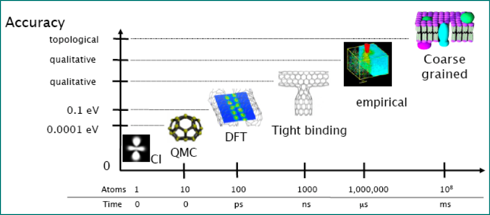
Motivation
- My examples are from atomistic materials modelling and electronic structure, but approach is general
- All the activities I'm interested in require robust, automated coupling of two or more codes
- For example, current projects include:
- developing and applying multiscale methods
- generating interatomic potentials
- uncertainty quantification
Atomic Simulation Environment (ASE)
- Within atomistic modelling, emerging standard for scripting interfaces is ASE
- Wide range of calculators, flexible (but not too flexible) data model for Atoms objects
- Can use many codes as drop-in replacements:

Atomic Simulation Environment (ASE)
- ASE mostly uses file-based interfaces: input generators and output parsers
- Collection of parsers aids validation and verification - cf. DFT $\Delta$-code project
- Coupling $N$ codes requires maintaining $N$ parsers/interfaces, rather than $N^2$ converters
- High-level functionality can be coded generically, or imported from other packages (e.g.
spglib,phonopy) using minimal ASE-compatible API
File-based interfaces vs. Native interfaces
- File-based interfaces (like those mostly used in ASE) to electronic structure codes can be slow and/or incomplete and parsers are hard to keep up to date and robust
- Standardised output (e.g. chemical markup language, XML, JSON) part of solution
- So are robust parsers - NoMaD Centre of Excellence has produced parsers for top ~40 electronic structure and atomistic codes
- Alternative: native interfaces provide a much deeper wrapping, exposing full public API of code to script writers (e.g. GPAW, LAMMPSlib)
- Future proofing: anything accessible from Python works with other high-level languages (e.g. Julia)
f90wrap adds derived type support to f2py
- Writing deep Python interfaces 'by hand' is possible but tedious
- There are good automatic interface generators for C++ codes (e.g.pybind11, SWIG, Boost.Python), but none support modern Fortran
- There's still lots of high-quality Fortran code around...
- f2py scans Fortran 77/90/95 codes, generates Python interfaces for individual routines
- No support for modern Fortran features: derived types, overloaded interfaces
- My
f90wrappackage addresses this by generating an additional layer of wrappers, adding support for derived types, module data, efficient array access, Python 2.6+ and 3.x
f90wrap schematic overview

More details: J. R. Kermode, f90wrap: an automated tool for constructing deep Python interfaces to modern Fortran codes. J. Phys. Condens. Matter (2020) doi:10.1088/1361-648X/ab82d2
Example: wrapping the bader code
- Widely used code for post-processing charge densities to construct Bader volumes
- Python interface would allow code to be used in workflows without I/O etc.
- Downloaded source, used
f90wrapto automatically generate a deep Python interface with very little manual work
Generation and compilation of wrappers:
f90wrap -v -k kind_map -I init.py -m bader \
     kind_mod.f90 matrix_mod.f90 \
     ions_mod.f90 options_mod.f90 charge_mod.f90 \
     chgcar_mod.f90 cube_mod.f90 io_mod.f90 \
     bader_mod.f90 voronoi_mod.f90 multipole_mod.f90

f2py-f90wrap -c -m _bader f90wrap_*.f90 -L. -lbader
To install it yourself, run the commands below, taking care to adjust PY_INSTALL_DIR according to your local setup:
git clone https://gitlab.com/jameskermode/bader
cd bader
export PY_INSTALL_DIR=~/.local/lib/python3.8/site-packages
make -f makefile.osx_gfortran python
Example: wrapping the bader code (contd.)
Restart a gpaw DFT calculation (or run if necessary) and retrieve the density:
import os
from ase.build import bulk
from gpaw import GPAW, restart

if not os.path.exists('si-vac.gpw'):
    si = bulk('Si', cubic=True)
    del si[0] # create a vacancy
    gpaw = GPAW(h=0.15)
    si.set_calculator(gpaw)
    si.get_potential_energy()
    gpaw.write('si-vac.gpw')

si, gpaw = restart('si-vac.gpw')
rho = gpaw.get_pseudo_density()
plt.plot(si.positions[:, 0], si.positions[:, 1], 'r.', ms=50)
plt.imshow(rho[:,:,0], extent=[0, si.cell[0,0], 0, si.cell[1,1]]);

import bader

bdr = bader.bader(si, rho)

print('ionchg:', bdr.ionchg)
ionchg: [4.2901335  4.43094328 4.28875689 4.43093625 4.32306902 4.43071537
 4.3392679 ]

  CALCULATING BADER CHARGE DISTRIBUTION
                 0  10  25  50  75  100
  PERCENT DONE:  **********************

  REFINING AUTOMATICALLY
  ITERATION: 2
  CHECKED POINTS:          0
  REASSIGNED POINTS:       0

  RUN TIME:       0.05 SECONDS

  CALCULATING MINIMUM DISTANCES TO ATOMS
                 0  10  25  50  75  100
  PERCENT DONE:  **********************

  RUN TIME:    0.01 SECONDS
## TAB-complete to introspect inside `bdr` Fortran type
dtype('float64')
# collect Bader volumes associated with atom #5
atom = 4
rho3 = np.zeros_like(rho)
for v in (bdr.nnion == atom+1).nonzero()[0]:
    rho3[bdr.volnum == v+1] = rho[bdr.volnum == v+1]
# write a CUBE file to allow visualisation of density (FIXME: can this be avoided?)
from ase.io.cube import write_cube

with open('rho3.cube', 'w') as f:
    write_cube(f, si, rho3)
import nglview
v = nglview.show_ase(si, gui=True)
v.add_representation('unitcell')
v.add_component('rho3.cube')
v.component_1.update_surface()
v
NGLWidget()
Tab(children=(Box(children=(Box(children=(Box(children=(Label(value='step'), IntSlider(value=1, min=-100)), la…
Wrapping Castep with f90wrap - CasPyTep
f90wrapcan now wrap large codes like Castep to provide deep access to internal data- Summer project in 2014 by Greg Corbett at STFC built proof-of-principle Castep/Python interface. Results described in RAL technical report
- Warwick MSc student Sebastian Potthoff wrote his dissertation on
CasPyTepin 2016, adding MPI support and optimising performance of Nudged Elastic Band algorithm, coded in Python - Since then I've extended a bit further - e.g. adding Python 3.x support
- Peter Byrne has very recently added a slimmed down
Castep_Pythonmodule with a high level API, also built usingf90wrap
CasPyTep Requirements
- Castep source code - tested with latest development version
- Supported Fortran compiler (tested with
gfortranandifort) - Python Python 3.6+
- Numpy:
pip install numpy - f90wrap package:
pip install f90wrap - Atomic Simulation Enviroment (ASE):
pip install ase
Compiling CasPyTep
In principle:
cd castep
make
make python
export PY_INSTALL_DIR=/usr/local/python3.7/site-packages # or somewhere else
make python-install
For the high level bindings only - see README.INSTALL for more details:
make castep_python
pip install -e obj/[ARCH]
CasPyTep Current Features
Set of source files currently wrapped is as follows, can be easily expanded:
  Utility:     constants.F90 algor.F90 comms.serial.F90
               io.F90 trace.F90 license.F90 buildinfo.f90
  Fundamental: parameters.F90 cell.F90 basis.F90
               ion.F90 density.F90 wave.F90
  Functional:  model.F90 electronic.F90 firstd.f90 xc.f90
Already far too much to wrap by hand:
- 35 kLOC Fortran and 55 kLOC Python auto-generated
- 23 derived types
- ~2600 subroutines/functions
What is wrapped?
- Dynamic introspection of data and objects:
- Module-level variables:
current_cell, etc (NB: must havetargetattribute) - Fortran derived types exposed as Python classes (e.g
unit_cell,model_state), including all elements, arrays, etc. within them - Arrays (including arrays of derived types) - no copying necessary to access data in numerical arrays e.g.
current_cell%ionic_positionsexposed directly in Python
- Module-level variables:
- Documentation strings are extracted from source code
io_abort()raisesRuntimeErrorexception- Plus, there's a minimal ASE-compatible high level calculator
CasPyTep(atoms)
Taking caspytep for a test drive
import numpy as np
import caspytep
## uncomment line below and press TAB for autocompletion
caspytep.
#caspytep.cell.unit_cell.
## append a ? to access documentation strings
caspytep.model.model_wave_read?
#caspytep.cell.cell_read?
Single point calculation
This uses the ASE-compatible interface provided by the CasPyTep class.
from ase.build import bulk

atoms = bulk('Si', cubic=True)
calc = caspytep.calculator.CasPyTep(atoms=atoms)
atoms.set_calculator(calc)
e = atoms.get_potential_energy()
f = atoms.get_forces()
print(f'energy: {e:.3f} eV')
print(f'forces: {f}')
energy: -1351.306 eV
forces: [[-1.77531190e-06  7.79031704e-06 -7.78323921e-06]
 [ 5.28965998e-05 -1.26374348e-05 -2.42809706e-05]
 [-4.99546145e-06  1.06564617e-05  5.72414230e-05]
 [-1.50490900e-05 -1.54993264e-05 -1.93367246e-06]
 [ 9.94049519e-06  3.30692511e-05 -7.02829293e-06]
 [-1.56277562e-05  7.36665153e-06 -1.61929791e-05]
 [ 1.36706212e-05 -1.19693116e-05  3.73698167e-05]
 [-3.90600967e-05 -1.87766085e-05 -3.73920853e-05]]
Interactive introspection
Unlike with standard ASE or other scripting approaches, after running a calculation, we can now poke around in all the internal arrays:
#calc.model.eigenvalues
#calc.model.cell.ionic_positions
#calc.model.cell.ionic_positions[...,0]
#calc.model.wvfn.beta_phi
#calc.model.cell.ionic_velocities.T
from ase.units import Hartree
calc.parameters.cut_off_energy
190.4797021705707
Postprocessing and Visualisation
from ase.units import Bohr
p = calc.model.cell.ionic_positions.copy()
p = p[:, :, 0] # first species only
p = calc.model.cell.real_lattice.T @ p
xi, yi, zi = p * Bohr
plt.scatter(xi, yi, s=200, c='r')
plt.axis([0, atoms.cell[0,0], 0, atoms.cell[1,1]]); plt.axis("scaled");

# overlay the charge density
plt.scatter(xi, yi, s=200, c='r')
den = calc.model.den.real_charge.copy()
basis = caspytep.basis.get_current_basis()
den3 = (den.reshape((basis.ngx, basis.ngy,
                     basis.ngz), order='F') /
        basis.total_grid_points)
plt.imshow(den3[:, :, basis.ngz//2],
           extent=[0, atoms.cell[0,0], 0, atoms.cell[1,1]]);

Updating data inside a running Castep instance
- So far this is just analysis/post-processing, but could easily go beyond this and steer calculations based on results of e.g. Bader analysis.
- In the simplest case, we can move the ions and continue the calculation without having to restart from scratch (or do any I/O of
.checkfiles etc.). - This allows embedded Castep to be efficiently used as a standard ASE calculator, with existing high-level algorithms: geometry optimisation, NEB, basin hopping, etc.
- Compared to file-based interface, save overhead of starting Castep each time
- Reuse electronic model from one ionic step to the next
- Wavefunction and charge density extrapolation possible just as in MD
Example 1 - geometry optimisation
from ase.build import bulk
from ase.optimize import LBFGS
from caspytep.calculator import CasPyTep

atoms = bulk("Si", cubic=True)
calc = CasPyTep(atoms=atoms)
atoms.set_calculator(calc)
atoms.rattle(0.01)
a0 = atoms.copy()
opt = LBFGS(atoms)
opt.run(fmax=0.1)
print(atoms.get_potential_energy())
       Step     Time          Energy         fmax
LBFGS:    0 15:45:59    -1351.292226        0.3984
LBFGS:    1 15:46:02    -1351.299107        0.2784
LBFGS:    2 15:46:05    -1351.306328        0.0425
-1351.3063283114898
Example 2 - testing new algorithms
Python interface makes it quick to try out new high-level algorithms or connect things in new ways, e.g. testing preconditioned geometry optimizer [Packwood2016]
from ase.optimize.precon import PreconLBFGS
from caspytep.calculator import CasPyTep

atoms = a0.copy() # restart from same randomised positions as above
atoms.set_calculator(CasPyTep(atoms=atoms))
opt = PreconLBFGS(atoms, precon='Exp')
opt.run(fmax=0.05)
PreconLBFGS:   0  15:46:42    -1351.292226       0.3984
PreconLBFGS:   1  15:46:51    -1351.306183       0.0593
PreconLBFGS:   2  15:46:54    -1351.306486       0.0182
True
Example 3 - convergence testing
This is an example of using the native CasPyTep interface directly rather than the ASE compatibility layer. We increase the plane wave cutoff energy in steps of 10% until energy changes by less than $10^{-3}$ Hartree. (This isn't necessarily the best way to do convergence testing...)
from ase.build import bulk
from caspytep.calculator import CasPyTep

calc = CasPyTep(atoms=bulk("Si")) # 2-atom Si system

energy_tol = 1e-4
current_params = caspytep.parameters.get_current_params()
current_params.cut_off_energy = 7.0

cutoffs = []
energy = []
while True:
    caspytep.basis.basis_initialise(current_params.cut_off_energy)
    current_params.fine_gmax = (current_params.fine_grid_scale *
                                np.sqrt(2.0*current_params.cut_off_energy))
    caspytep.ion.ion_real_initialise()
    model = caspytep.model.model_state()
    model.converged = caspytep.electronic.electronic_minimisation(model)
    current_params.cut_off_energy *= 1.1
    print('cutoff %.2f energy %.5f' % (current_params.cut_off_energy,
                                       model.total_energy))
    cutoffs.append(current_params.cut_off_energy)
    energy.append(model.total_energy)
    if len(energy) > 2 and abs(energy[-1] - energy[-2]) < energy_tol:
        print('converged at cutoff', cutoffs[-1])
        break
cutoff 7.70 energy -12.42124
cutoff 8.47 energy -12.42233
cutoff 9.32 energy -12.42250
cutoff 10.25 energy -12.42281
cutoff 11.27 energy -12.42289
converged at cutoff 11.273570000000007
from ase.units import Hartree

ecut = np.array(cutoffs) * Hartree
ediff = np.array(energy) * Hartree
ediff -= ediff[-1]
plt.plot(ecut, abs(ediff) * 1e3 / caspytep.cell.current_cell.num_ions, 'o-')
plt.xlabel('Cutoff / eV')
plt.ylabel('Energy Error / meV')
plt.axhline(1, linestyle='--');

Missing features
- Make more example scripts and notebooks, e.g.:
- MD with wavefunction extrapolation
- Introspection and visualisation of wavefunctions/densities in situ
- Integrate with your favourite post-processing/analysis tools - e.g. OptaPyDOS
- Improve Castep re-entrancy to allow multiple models/cells (partially done?)
- e.g. allow
current_cellto be updated in place without having to callcell_read():
cell_read()intocell_read()andcell_initialise() - e.g. allow
- Think more about what to reset when configuration changes...
- e.g. symmetry operations may need to be updated when ions move
- Experiment with MPI parallelisation and benchmark wrt standard Castep
mpirun -np N python script.pyworks if CasPyTep compiled with MPI libraries
Over to you...
Download the image and have a play with CasPyTep in the practical session.
Install Docker CE (free download) on your Linux/Mac/Windows machine (root access required), then:
gzcat caspytep.tar.gz | docker load
docker run -v ~:/root/host -p 8899:8899 caspytep
Then point your web brower at http://localhost:8899 and browse to noteboooks > demo.ipynb to open this notebook.
To open a bash shell instead:
docker run -v ~:/root/host -it caspytep /bin/bash
$ python
>>> import caspytep
Summary - Benefits of Scripting Interfaces
Primary:
- Automated preparation of input files
- Analysis and post-processing
- Batch processing
Secondary:
- Expand access to advanced features to less experienced programmers
- Simplify top-level programs
- Unit and regression testing framework
Longer term benefits:
- Encourages good software engineering in main code - modularity, well defined APIs
- Speed up development of new algorithms by using an appropriate mixture of high- and low-level languages
Conclusions and Outlook
- Scripting interfaces can be very useful for automating calculations, or connecting components in new ways
- Can give legacy C/Fortran code a new lease of life
- Provides interactive environment for testing, debugging, development and visualisation
- Appropriate mix of high- and low-level languages maximses overall efficiency
- Julia is shaking up this balance a bit