Scikit-Learn: Machine Learning in the Python ecosystem
MLOSS workshop - NIPS 2013
December 10, 2013
Gilles Louppe ([@glouppe](https://twitter.com/glouppe))
(with Gaël Varoquaux ([@GaelVaroquaux](https://twitter.com/GaelVaroquaux))
and Andreas Müller ([@t3kcit](https://twitter.com/t3kcit)) as backups)
Scikit-Learn
- Machine learning library written in Python
- Simple and efficient, for both experts and non-experts
- Classical, well-established machine learning algorithms
- BSD 3 license
Overview
Supervised learning:
- Linear models (Ridge, Lasso, Elastic Net, ...)
- Ensemble methods (Random Forests, Bagging, GBRT, ...)
- Support Vector Machines
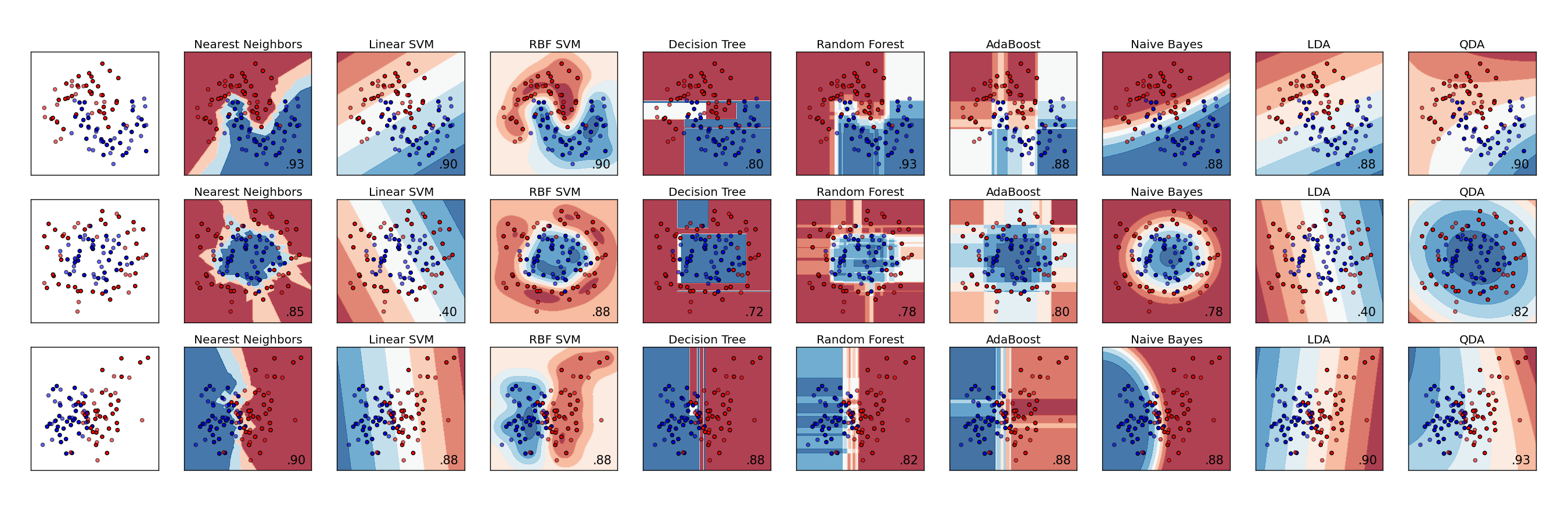 A comparison of (some of the) classifiers in Scikit-Learn
Unsupervised learning:
- Clustering (KMeans, Ward, ...)
- Matrix decomposition (PCA, ICA, ...)
- Outlier detection
Model selection and evaluation:
- Cross-validation
- Grid-search
- Lots of metrics
... and many more! (See our Reference)
Collaborative development
- 10~ core developers (mostly researchers)
- 100+ occasional contributors
- All working together on GitHub
- Emphasis on keeping the project maintainable
- Style consistency
- Unit-test coverage
- Documentation and examples
- Code review
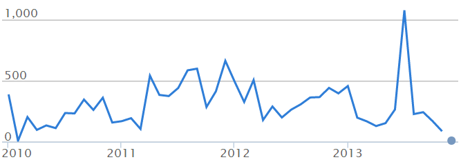
Number of commits:
Lines of code:
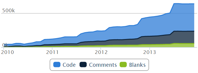
(Graphs generated by Ohloh.net)
A simple and unified API
All objects in scikit-learn share a uniform and limited API consisting of three complementary interfaces:
- an
estimatorinterface for building and fitting models; - a
predictorinterface for making predictions; - a
transformerinterface for converting data.
All of them takes as input data which is structured as Numpy arrays.
# Load data
from sklearn.datasets import load_digits
data = load_digits()
X, y = data.data, data.target

print X
print X.shape
print X.dtype
[[  0.   0.   5. ...,   0.   0.   0.]
 [  0.   0.   0. ...,  10.   0.   0.]
 [  0.   0.   0. ...,  16.   9.   0.]
 ...,
 [  0.   0.   1. ...,   6.   0.   0.]
 [  0.   0.   2. ...,  12.   0.   0.]
 [  0.   0.  10. ...,  12.   1.   0.]]
(1797, 64)
float64
Consistency across the package makes scikit-learn very usable in practice. Experimenting with different learning algorithms is as simple as changing a class definition.
# Instantiate a classifier
from sklearn.tree import DecisionTreeClassifier # Change this
clf = DecisionTreeClassifier()                  # ... and that

# Do stuff (and rely on the common interface across estimators)
from sklearn.pipeline import Pipeline
from sklearn.decomposition import PCA
from sklearn.cross_validation import cross_val_score

pipeline = Pipeline([("pca", PCA(n_components=10)),
                     ("classifier", clf)])

print "Accuracy =", cross_val_score(pipeline, X, y, cv=3).mean()
Accuracy = 0.803544498721
Through composition interfaces (e.g., Pipeline and FeatureUnion), the library also offers powerful mechanisms to express a wide variety of learning tasks within a small amount of code.
Finally, through duck-typing, the consistent API leads to a library that is easily extensible. It allows user-defined estimators to be easily incorporated into the Scikit-Learn workflow without any explicit object inheritance.
Integration in the scientific Python ecosystem
- The open source Python ecosystem provides a standalone, versatile and powerful scientific working environment, including:
- NumPy (for efficient manipulation of multi-dimensional arrays);
- SciPy (for specialized data structures (e.g., sparse matrices) and lower-level scientific algorithms),
- IPython (for interactive exploration),
- Matplotlib (for vizualization)
- Pandas (for data management and data analysis)
- (and many others...)
- Scikit-Learn builds upon NumPy and SciPy and complements this scientific environment with machine learning algorithms;
- By design, Scikit-Learn is non-intrusive, easy to use and easy to combine with other libraries.
End-to-end proof of concept
Let us illustrate the various components of the scientific Python ecosystem for the analysis of scientific data.
We consider genetic data from the HapMap project which catalogs common genetic variants in human beings from different populations in different parts of the world.
Genetics 101. The DNA in our cells are made of long chains of 4 chemical building blocks (adenine, thymine, cytosine, and guanine) which are strung together in 23 pairs of chromosomes. These genetic sequences contain information that influences our physical traits, our likelihood of suffering from disease, or the responses of our bodies to substances that we encounter in the environment.
The genetic sequences of different people are remarkably similar. When the chromosomes of two humans are compared, their DNA sequences can be identical for hundreds of bases. But at about one in every 1200 bases, on average, the sequences differ. These genetic differences are known as single nucleotide polymorphisms (SNPs). By identifying most of the approximately 10 million SNPs estimated to occur commonly in the human genome, the HapMap Project is identifying the basis for a large fraction of the genetic diversity in the human species.
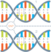
DNA sequences 1 and 2 are similar to each other,
except at some specific locations called _SNPs_.
The HapMap data includes genotypes for 1417 individuals, from 11 human populations from different parts of the world (e.g., Europe, Africa, Asia; see Appendix A). It regroups genotypes for all SNPs (from all 23 chromosomes) reported by the HapMap genotyping centers.
From a data management point of view, the HashMap data comes with many of the hurdles of real-world data:
- It is scattered in a large collection of genotype data files (one per chromosome/population);
- It is large (1417 individuals, millions of SNPs; GBs of raw data);
- SNPs are not all reported for all populations;
- Genotypes are sometimes missing;
- Values are heterogeneous (numbers, strings, symbols).
We will explore and analyze the HapMap data directly from this IPython session.
IPythonprovides an interactive web-based working environment (called Notebook) combining code execution, text, plots and media into a single document.
Caution! The following analysis is merely an illustration of the capabilities of the Python ecosystem. Don't draw any scientific conclusions from it.
a) Downloading the data
Besides Python code, IPython also allows for the execution of arbitrary bash commands, which extends the Python ecosystem with all tools available from the command line.
%%bash
# Load the data from chromosome 15
mkdir -p data
wget -P data http://hapmap.ncbi.nlm.nih.gov/downloads/genotypes/2010-08_phaseII+III/forward/genotypes_chr15_ASW_r28_nr.b36_fwd.txt.gz
wget -P data http://hapmap.ncbi.nlm.nih.gov/downloads/genotypes/2010-08_phaseII+III/forward/genotypes_chr15_CEU_r28_nr.b36_fwd.txt.gz
wget -P data http://hapmap.ncbi.nlm.nih.gov/downloads/genotypes/2010-08_phaseII+III/forward/genotypes_chr15_CHB_r28_nr.b36_fwd.txt.gz
wget -P data http://hapmap.ncbi.nlm.nih.gov/downloads/genotypes/2010-08_phaseII+III/forward/genotypes_chr15_CHD_r28_nr.b36_fwd.txt.gz
wget -P data http://hapmap.ncbi.nlm.nih.gov/downloads/genotypes/2010-08_phaseII+III/forward/genotypes_chr15_GIH_r28_nr.b36_fwd.txt.gz
wget -P data http://hapmap.ncbi.nlm.nih.gov/downloads/genotypes/2010-08_phaseII+III/forward/genotypes_chr15_JPT_r28_nr.b36_fwd.txt.gz
wget -P data http://hapmap.ncbi.nlm.nih.gov/downloads/genotypes/2010-08_phaseII+III/forward/genotypes_chr15_LWK_r28_nr.b36_fwd.txt.gz
wget -P data http://hapmap.ncbi.nlm.nih.gov/downloads/genotypes/2010-08_phaseII+III/forward/genotypes_chr15_MEX_r28_nr.b36_fwd.txt.gz
wget -P data http://hapmap.ncbi.nlm.nih.gov/downloads/genotypes/2010-08_phaseII+III/forward/genotypes_chr15_MKK_r28_nr.b36_fwd.txt.gz
wget -P data http://hapmap.ncbi.nlm.nih.gov/downloads/genotypes/2010-08_phaseII+III/forward/genotypes_chr15_TSI_r28_nr.b36_fwd.txt.gz
wget -P data http://hapmap.ncbi.nlm.nih.gov/downloads/genotypes/2010-08_phaseII+III/forward/genotypes_chr15_YRI_r28_nr.b36_fwd.txt.gz
for f in data/*.gz; do gunzip $f; done
# Look at the 3 first lines of the data
!head -n 3 data/genotypes_chr15_ASW_r28_nr.b36_fwd.txt
rs# alleles chrom pos strand assembly# center protLSID assayLSID panelLSID QCcode NA19625 NA19700 NA19701 NA19702 NA19703 NA19704 NA19705 NA19708 NA19712 NA19711 NA19818 NA19819 NA19828 NA19835 NA19834 NA19836 NA19902 NA19901 NA19900 NA19904 NA19919 NA19908 NA19909 NA19914 NA19915 NA19916 NA19917 NA19918 NA19921 NA20129 NA19713 NA19982 NA19983 NA19714 NA19985 NA19984 NA20128 NA20126 NA20127 NA20277 NA20276 NA20279 NA20282 NA20281 NA20284 NA20287 NA20288 NA20290 NA20289 NA20291 NA20292 NA20295 NA20294 NA20297 NA20300 NA20298 NA20301 NA20302 NA20317 NA20319 NA20322 NA20333 NA20332 NA20335 NA20334 NA20337 NA20336 NA20340 NA20341 NA20343 NA20342 NA20344 NA20345 NA20346 NA20347 NA20348 NA20349 NA20350 NA20351 NA20357 NA20356 NA20358 NA20359 NA20360 NA20363 NA20364 NA20412
rs7494890 C/T chr15 18275409 + ncbi_b36 sanger urn:LSID:illumina.hapmap.org:Protocol:Human_1M_BeadChip:3 urn:LSID:sanger.hapmap.org:Assay:H1Mrs7494890:3 urn:lsid:dcc.hapmap.org:Panel:US_African-30-trios:4 QC+ TT TT TT TT TT TT TT TT TT CT TT CT CT TT CT TT TT TT TT TT TT TT TT TT TT CT TT CT CT CT TT TT TT TT TT TT TT TT TT TT TT TT TT CT TT TT TT TT TT TT TT TT TT TT TT TT CT CT TT TT TT TT TT TT TT TT TT TT TT TT TT TT TT TT TT TT TT TT TT TT TT TT CT CC TT TT TT
rs12900938 C/T chr15 18294933 + ncbi_b36 sanger urn:LSID:illumina.hapmap.org:Protocol:Human_1M_BeadChip:3 urn:LSID:sanger.hapmap.org:Assay:H1Mrs12900938:3 urn:lsid:dcc.hapmap.org:Panel:US_African-30-trios:4 QC+ CT CT TT TT CT TT TT TT CT TT TT TT TT TT TT TT TT TT TT CT TT TT TT CT TT TT TT TT TT TT CT TT TT CT CT CT TT TT TT TT CT CT TT TT TT TT TT TT TT TT TT CC NN TT CT TT TT TT TT TT CT TT TT TT CT TT TT TT TT CT CT TT TT TT TT TT TT TT CT TT CT TT TT TT TT TT TT
b) Data preprocessing with pandas and sklearn
Scikit-Learn expects input data to be represented as two-dimensional NumPy arrays of numerical values. In our case, the HapMap data is not represented in this way and needs to be preprocessed to conform to our standards.
We rely on the pandas module for loading, converting and merging the datafiles into a single NumPy array.
The
pandasmodule aims at providing fast, flexible and expressive data structures designed to make working with labeled or relational data both easy and intuitive. It is one of the most powerful and flexible Python packages for data manipulation. In particular,pandasintegrates into the scientific Python ecosystem by providing NumPy-compatible data structures and tools for easily converting data from one format to another.
import numpy as np
import pandas as pd

def load_genotypes(filename, population):
    # Load the data into a dataframe
    df = pd.read_csv(filename, sep=" ", index_col=0)

    # Map genotypes to 0-1-2 values
    mask = df.alleles == 'A/C'
    df[mask] = df[mask].replace(to_replace=['AA', 'AC', 'CC'],
                                value=[0, 1, 2])
    mask = df.alleles == 'A/G'
    df[mask] = df[mask].replace(to_replace=['AA', 'AG', 'GG'],
                                value=[0, 1, 2])
    mask = df.alleles == 'A/T'
    df[mask] = df[mask].replace(to_replace=['AA', 'AT', 'TT'],
                                value=[0, 1, 2])
    mask = df.alleles == 'C/G'
    df[mask] = df[mask].replace(to_replace=['CC', 'CG', 'GG'],
                                value=[0, 1, 2])
    mask = df.alleles == 'C/T'
    df[mask] = df[mask].replace(to_replace=['CC', 'CT', 'TT'],
                                value=[0, 1, 2])
    mask = df.alleles == 'G/T'
    df[mask] = df[mask].replace(to_replace=['GG', 'GT', 'TT'],
                                value=[0, 1, 2])

    # Replace missing value placeholders
    df.replace(to_replace='NN', value=-1, inplace=True)

    # Copy data into a new frame
    individuals = df.columns[10:]
    snps = df.index

    new_df = pd.DataFrame(index=individuals)
    new_df["population"] = population
    new_df[snps] = df[individuals].T
    new_df = new_df.convert_objects()

    # Drop SNPs corresponding to deletions/insertions
    new_df = new_df.drop(new_df.columns[new_df.dtypes == "object"][1:], axis=1)

    return new_df

# Concatenate all files and only keep common SNPs
filename = "genotypes_chr15_%s_r28_nr.b36_fwd.txt"
populations = ["ASW", "CEU", "CHB", "CHD", "GIH", "JPT",
               "LWK", "MEX", "MKK", "TSI", "YRI"]

df = pd.concat([load_genotypes(filename % population, population)
                    for population in populations],
               join="inner")

# Convert to Numpy arrays
snps = df.columns[1:]
X = df[snps].values.astype(np.int8)
y = df["population"].values.astype(np.str)

# Save for later
np.savez("data/chr15-all-numpy.npz", X=X, y=y, snps=snps)

# Warning! This takes long...
# To save time, let us load the binary files generated above
import numpy as np

data = np.load("data/chr15-all-numpy.npz")
snps = data["snps"]
X = data["X"]
y = data["y"]
print "SNPs =", snps[:10]
print "X =", X
print "X.shape =", X.shape
print "y =", y
SNPs = Index([u'rs7494890', u'rs12900938', u'rs12905389', u'rs10163108', u'rs6599770', u'rs7171651', u'rs7170864', u'rs12440100', u'rs10152550', u'rs12906138'], dtype=object)
X = [[2 1 2 ..., 1 1 1]
 [2 1 2 ..., 1 0 1]
 [2 2 2 ..., 2 1 2]
 ...,
 [1 2 1 ..., 1 0 1]
 [2 2 2 ..., 2 2 2]
 [1 2 1 ..., 2 1 2]]
X.shape = (1417, 33800)
y = ['ASW' 'ASW' 'ASW' ..., 'YRI' 'YRI' 'YRI']
# Limit to 3000 SNPs for faster interactions
snps = snps[:3000]
X = X[:, :3000]
Data is now converted to NumPy arrays. However, it still contains missing values (marked as -1) that need to be filled before being fed to Scikit-Learn estimators.
As a last preprocessing step, we rely on tools from the sklearn.preprocessing submodule to replace missing values.
The
sklearn.preprocessingsubmodule includes algorithms for encoding, normalizing or imputing data. All are offered as transformers.
print "Before imputation:", np.unique(X)

from sklearn.preprocessing import Imputer
imputer = Imputer(missing_values=-1, strategy="most_frequent")
X = imputer.fit_transform(X)

print "After imputation:", np.unique(X)
Before imputation: [-1  0  1  2]
After imputation: [ 0.  1.  2.]
c) Data visualization with matplotlib
In exploratory analysis, data visualization plays an important role in identifying interesting patterns. Representing your data graphically allows to visualize quantities and relationships that are otherwise difficult to interpret. In particular, when tackling a new problem, visualization often helps to quickly grasp what is going on in the data.
We rely on the matplotlib module for generating our figures and plots.
The
matplotlibmodule is a plotting library for producing high-quality figures with fine-grained layout control. It integrates into the IPython shell (à la MATLAB) to provide an interactive environement.
# Project the data to a 2D space for visualization
from sklearn.decomposition import RandomizedPCA
Xp = RandomizedPCA(n_components=2, random_state=1).fit_transform(X)
# Setup matplotlib to work interactively
%matplotlib inline
from matplotlib import pyplot as plt

# Plot individuals
populations = np.unique(y)
colors = plt.get_cmap("hsv")
plt.figure(figsize=(10, 4))

for i, p in enumerate(populations):
    mask = (y == p)
    plt.scatter(Xp[mask, 0], Xp[mask, 1],
                c=colors(1. * i / 11), label=p)

plt.xlim([-30, 50])
plt.legend(loc="best")
plt.show()

In this plot, we observe that individuals from a same population are clustered together, which confirms that they share the same genetic variants.
We also observe that some populations are grouped together into larger clusters (Asian people (CHN, CHD, JPT); African people (MKK, LWK, YRI); Caucasian people (CEU, TSI)), which suggests that individuals from those populations share common ancestors.
d) Learn from the data with sklearn
We now consider the learning task that consists in predicting the population of an individual given his genotype.
Let us first learn a simple linear model.
from sklearn.cross_validation import train_test_split
X_train, X_test, y_train, y_test = train_test_split(X, y, random_state=1)

from sklearn.linear_model import RidgeClassifierCV
clf = RidgeClassifierCV().fit(X_train, y_train)
clf.score(X_test, y_test)
0.63098591549295779
from sklearn.metrics import confusion_matrix

def print_cm(cm, labels):
    # Nicely print the confusion matrix
    print " " * 4,
    for label in labels:
        print " %s" % label,
    print

    for i, label1 in enumerate(labels):
        print label1,
        for j, label2 in enumerate(labels):
            print "%4d" % cm[i, j],
        print

print_cm(confusion_matrix(y_test,
                          clf.predict(X_test),
                          labels=populations), populations)
      ASW  CEU  CHB  CHD  GIH  JPT  LWK  MEX  MKK  TSI  YRI
ASW   12    3    0    0    0    1    0    0    0    0    6
CEU    0   30    3    0    0    3    0    2    0    4    2
CHB    0    4   11    8    0    8    0    0    0    0    2
CHD    0    3    7   13    0    3    0    0    0    0    1
GIH    0    2    0    0   23    1    0    0    0    2    0
JPT    0    0    9    4    0   18    0    0    0    0    0
LWK    2    0    1    1    0    1   16    0    4    1    8
MEX    0    0    0    2    0    0    0   15    0    0    0
MKK    0    2    0    0    0    0    1    0   41    0    1
TSI    0   12    3    0    0    0    0    4    0    9    0
YRI    2    3    2    0    0    1    1    0    1    0   36
By examining the confusion matrix, we observe that errors mainly happen within the larger clusters previously highlighted. For example, people from Tuscany (TSI) are often wrongly predicted as Utah residents (CEU) - both indeed have European ancestors and were clustered together - but are never as people from Asia.
Let us now examine the coefficients of the learned model.
# Plot coefficients
coef = np.mean(np.abs(clf.coef_), axis=0)

plt.figure(figsize=(10, 4))
plt.bar(range(len(snps)), coef)
plt.show()

# Top 10 SNPs
indices = np.argsort(coef)[::-1]

for i in range(10):
    print coef[indices[i]], snps[indices[i]]

0.0848131341116 rs6497292
0.0836956330076 rs10451027
0.0806013765047 rs10152550
0.076076994518 rs4887567
0.0719622014853 rs7161804
0.0718253208302 rs4906820
0.0616491365731 rs12900228
0.0597368222807 rs6602936
0.0558123165311 rs7164409
0.0545777401193 rs8034210
As indicated by dbSNP, rs6497292 happens to be located in gene HERC2 (8924), known to be associated with skin/hair/eye pigmentation variability. It is therefore not surprising to find this SNP at the top of the ranking.
The same kind of analysis can be carried out with other models from Scikit-Learn. For example, using a forest of randomized trees yields the following results:
from sklearn.ensemble import ExtraTreesClassifier
clf = ExtraTreesClassifier(n_estimators=100,
                           max_features=0.2,
                           n_jobs=2,
                           random_state=1).fit(X_train, y_train)
clf.score(X_test, y_test)
0.73802816901408452
print_cm(confusion_matrix(y_test,
                          clf.predict(X_test),
                          labels=populations), populations)
      ASW  CEU  CHB  CHD  GIH  JPT  LWK  MEX  MKK  TSI  YRI
ASW    3    0    0    0    0    0    0    1    6    0   12
CEU    0   43    0    0    0    0    0    0    0    1    0
CHB    0    0   21   12    0    0    0    0    0    0    0
CHD    0    0    1   25    0    1    0    0    0    0    0
GIH    0    3    0    0   23    0    0    0    0    2    0
JPT    0    0    1    9    0   21    0    0    0    0    0
LWK    0    0    0    0    0    0   13    0    8    0   13
MEX    0    4    0    1    0    0    0   10    0    2    0
MKK    0    0    0    0    0    0    0    0   45    0    0
TSI    0   15    0    0    1    0    0    0    0   12    0
YRI    0    0    0    0    0    0    0    0    0    0   46
# Plot importances
importances = clf.feature_importances_

plt.figure(figsize=(10, 4))
plt.bar(range(len(snps)), importances)
plt.show()

# Top 10 SNPs
indices = np.argsort(importances)[::-1]

for i in range(10):
    print importances[indices[i]], snps[indices[i]]

0.017715578803 rs1800410
0.01274291206 rs728404
0.0121761568447 rs2719921
0.0105565204679 rs3883068
0.010513859461 rs2739811
0.0104700121838 rs4932620
0.0101585372114 rs2739804
0.00921181949862 rs12593141
0.00900805253712 rs6497292
0.0081780757186 rs2719923
Results are not the same as previously. However SNPs that are reported are still meaningful: rs1800410 is located within gene OCA2 (4948), known to be associated with oculocutaneous (eyes and skin) albinism.
Overall, this suggests that there is no single SNP responsible alone for how populations look. Instead, and as expected, traits are dilluted all along the genome and there exist multiple genetic variants that can be used to identify an individual.
Conclusions
Python data-oriented packages tend to complement and integrate smoothly with each other. Together, they provide a powerful, flexible and coherent working environment for real-world scientific data analysis.
Scikit-Learn complements this ecosystem with machine learning algorithms and data analysis utilities.
Appendix A: Populations from the HapMap data
- ASW: African ancestry in Southwest USA
- CEU: Utah residents with Northern and Western European ancestry from the CEPH collection
- CHB: Han Chinese in Beijing, China
- CHD: Chinese in Metropolitan Denver, Colorado
- GIH: Gujarati Indians in Houston, Texas
- JPT: Japanese in Tokyo, Japan
- LWK: Luhya in Webuye, Kenya
- MEX: Mexican ancestry in Los Angeles, California
- MKK: Maasai in Kinyawa, Kenya
- TSI: Tuscan in Italy
- YRI: Yoruban in Ibadan, Nigeria (West Africa)