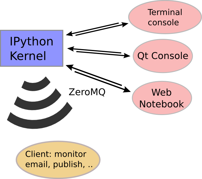
IPython
A multi-language architecture for interactive computing
[ipython.org](http://ipython.org)
Fernando Pérez
[fperez.org](http://fperez.org), [@fperez_org](http://twitter.com/fperez_org)
U.C. Berkeley
In [1]:
%pylab inline
%run talktools
Populating the interactive namespace from numpy and matplotlib
Hamming '62
The Lifecycle of a Scientific Idea (schematically)
- Individual exploratory work
- Collaborative development
- Parallel production runs (HPC, cloud, ...)
- Publication (with reproducible results!)
- Education
- Goto 1.
## 2001, instead of a Physics dissertation
## 2010, E Patterson, Enthought (key support!)
## T. Matev, T. Alatalo, R. Kern, Min RK, J. Gao, B. Granger
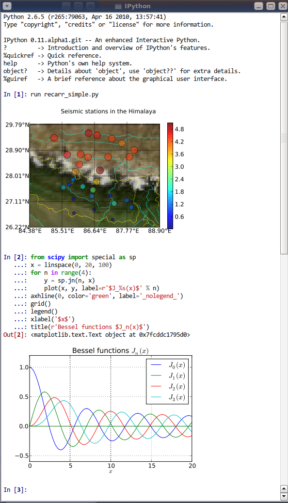
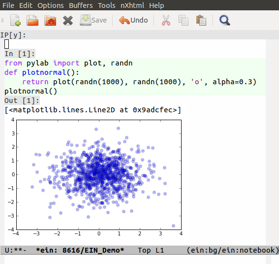
In [2]:
import scipy.special as spec
x = linspace(0, 20, 200)
for n in range(0,13,3):
    plot(x, spec.jn(n, x), label=r'$J_{%i}(x)$' % n)
grid()
legend()
title('Bessel Functions are neat');

Explore parameters interactively
In [4]:
@interactive(x=(1, 10))
def f(x):
    print 'X is:', x
X is: 5
In [5]:
from sklearn import datasets

digits = datasets.load_digits()
n = len(digits.images)

@interactive(i=(0,n-1))
def view_image(i):
    print 'Classif. Label:', digits.target[i]
    plt.matshow(digits.images[i], cmap=cm.gray_r)
    plt.show()
Classif. Label: 8

In [6]:
Image('fig/logo.png')
Out[6]:

In [7]:
Video('fig/animation.m4v') # Credit: Chris Kees, Army ERDC; created with Proteus.
Out[7]:
Browser multimedia + scientific visualization
In [8]:
plot_audio('voice.wav')
Audio('voice.wav')

Out[8]:
voice.wav:
LaTeX and symbolic mathematics support
In [9]:
Math(r'F(k) = \int_{-\infty}^{\infty} f(x) e^{2\pi i k} dx')
Out[9]:
$$F(k) = \int_{-\infty}^{\infty} f(x) e^{2\pi i k} dx$$
In [10]:
from sympy import symbols, Eq, factor, init_printing, expand
init_printing(use_latex=True)
x, y = symbols("x y")
In [11]:
eq = ((x+y)**3 * (x+1))
display(Eq(eq, expand(eq)))
$$\left(x + 1\right) \left(x + y\right)^{3} = x^{4} + 3 x^{3} y + x^{3} + 3 x^{2} y^{2} + 3 x^{2} y + x y^{3} + 3 x y^{2} + y^{3}$$
In [12]:
@interactive(n=(1,10))
def _(n):
    eq = ((x+y)**n * (x+1))
    display(Eq(eq, expand(eq)))
$$\left(x + 1\right) \left(x + y\right)^{5} = x^{6} + 5 x^{5} y + x^{5} + 10 x^{4} y^{2} + 5 x^{4} y + 10 x^{3} y^{3} + 10 x^{3} y^{2} + 5 x^{2} y^{4} + 10 x^{2} y^{3} + x y^{5} + 5 x y^{4} + y^{5}$$
Dynamic graph visualizations with D3
Talk to other languages: R (or Octave)
In [13]:
X = np.array([0,1,2,3,4])
Y = np.array([3,5,4,6,7])
# Now, load R support
%load_ext rmagic
In [14]:
%%R -i X,Y -o XYcoef
XYlm = lm(Y~X)
XYcoef = coef(XYlm)
print(summary(XYlm))
par(mfrow=c(2,2))
plot(XYlm)
Call:
lm(formula = Y ~ X)

Residuals:
   1    2    3    4    5
-0.2  0.9 -1.0  0.1  0.2

Coefficients:
            Estimate Std. Error t value Pr(>|t|)
(Intercept)   3.2000     0.6164   5.191   0.0139 *
X             0.9000     0.2517   3.576   0.0374 *
---
Signif. codes:  0 ‘***’ 0.001 ‘**’ 0.01 ‘*’ 0.05 ‘.’ 0.1 ‘ ’ 1

Residual standard error: 0.7958 on 3 degrees of freedom
Multiple R-squared:   0.81,	Adjusted R-squared:  0.7467
F-statistic: 12.79 on 1 and 3 DF,  p-value: 0.03739

Julia: seamless 2-way communication
In [15]:
%load_ext julia.magic
%julia @pyimport matplotlib.pyplot as plt
%julia @pyimport numpy as np
Initializing Julia interpreter. This may take some time...
In [16]:
%%julia
# Note how we mix numpy and julia:
x = linspace(0,2*pi,1000); # use the julia linspace
y = sin(3*x + 4*np.cos(2*x)); # use the numpy cosine and julia sine
plt.plot(x, y, color="red", linewidth=2.0, linestyle="--")
Out[16]:
[Line2D(_line0)]

In [17]:
jfib = %julia jfib(n, fib) = n < 2 ? n : fib(n-1, jfib) + fib(n-2, jfib)

def pyfib(n, fib):
    if n < 2:
         return n
    return fib(n-1, pyfib) + fib(n-2, pyfib)

pyfib(20, jfib)   # Credit: Steven Johnson, MIT.
Out[17]:

Fortran integration
In [18]:
%load_ext fortranmagic
In [22]:
%%fortran
subroutine f1(x, y, n)
    real, intent(in), dimension(n) :: x
    real, intent(out), dimension(n) :: y
    !intent(hide) :: n
    y = sin(x**2)
end subroutine f1
In [23]:
x = np.linspace(0, 2*pi, 300)
plot(x, f1(x));

- Library for format conversions
- HTML, LaTeX, PDF output.
- Basic command-line usage.
- Rich customization possibilities.
## Matthias Bussonnier, 2012
In [24]:
website('nbviewer.ipython.org')
Out[24]:
## Min RK, Brian, Greg Caporaso, Rob Knight (group), Justin Riley
In [25]:
website('http://www.nature.com/ismej/journal/v7/n3/full/ismej2012123a.html', 'Paper:')
Out[25]:
Notebooks and AMI for reproducibility:
In [26]:
website('http://qiime.org/home_static/nih-cloud-apr2012', 'Companion Website:')
Out[26]:
## Jake VanderPlas (astronomy/ML at UW)
In [27]:
website('http://jakevdp.github.io/blog/2013/12/05/static-interactive-widgets',
        'Pythonic Perambulations')
Out[27]:
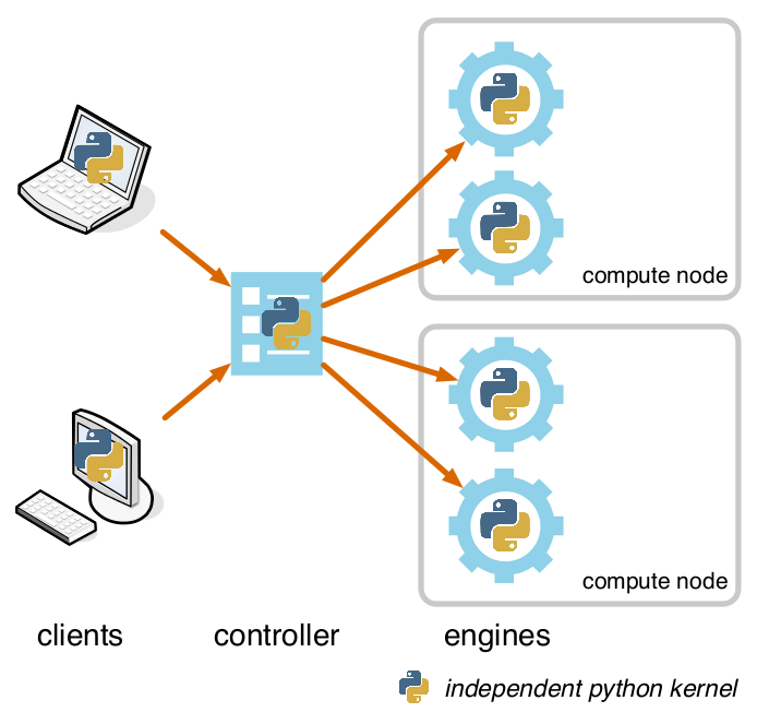
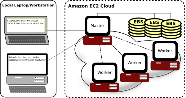
Using Notebook and IPython.parallel
- From: 8000 lines of Java, JS and HTML5, 2min/query
- To: 200 lines of Python, 2sec/query
In [28]:
YouTubeVideo('tlontoyWX70',start='800', width=600, height=400)
Out[28]:
Python for Signal Processing, By Jose Unpingco
|
|
By [Cam Davidson Pilon](http://www.camdp.com).
In [29]:
website('camdavidsonpilon.github.io/Probabilistic-Programming-and-Bayesian-Methods-for-Hackers',
        'Probabilistic programming...')
Out[29]:
By [Matthew Russell](https://github.com/ptwobrussell).
|
|
CS 109: Data Science at Harvard
In [30]:
website('http://cs109.org/homework/homework.php', 'CS 109 Homeworks')
Out[30]:
A growing (and amazing) body of work
For much more: [http://ipython.org/gallery](http://ipython.org/gallery)
IPython.parallel
# A healthy ecosystem, OSS and commercial
Enthought Canopy
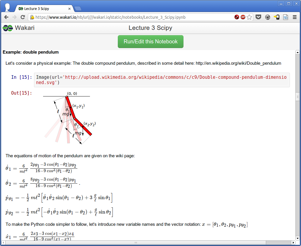
Continuum Analytics: Wakari
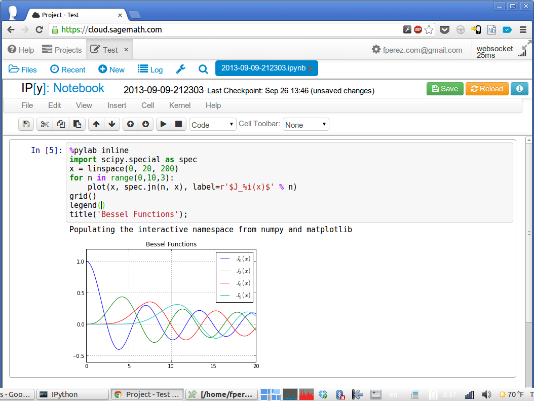
Cloud.sagemath.com: UW startup, W. Stein
Plot.ly: interactive JS plots in Python
In [31]:
website('http://nbviewer.ipython.org/gist/jackparmer/7729584', 'Rosling Countries',
        width=900, height=600)
Out[31]:
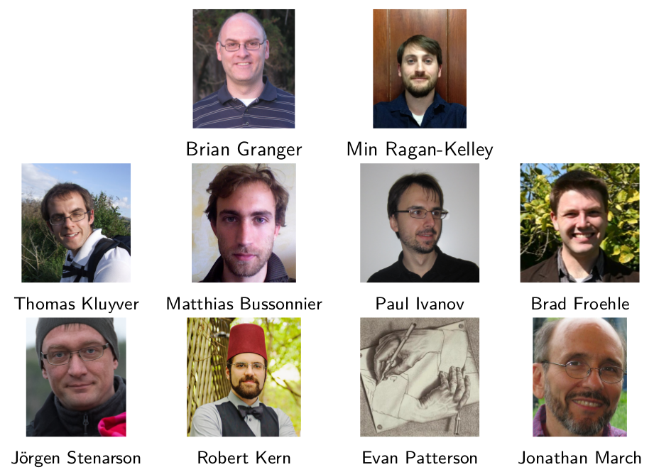
An incomplete cast of characters
- Brian Granger - Physics, Cal State San Luis Obispo
- Min Ragan-Kelley - Nuclear Engineering, UC Berkeley
- Matthias Bussonnier - Physics, Institut Curie, Paris
- Jonathan March- Enthought
- Thomas Kluyver - Biology, U. Sheffield
- Jörgen Stenarson - Elect. Engineering, Sweden.
- Paul Ivanov - Neuroscience, UC Berkeley.
- Robert Kern - Enthought
- Evan Patterson - Physics, Caltech/Enthought
- Brad Froehle - Mathematics, UC Berkeley
- Stefan van der Walt - UC Berkeley
- John Hunter - TradeLink Securities, Chicago.
- Prabhu Ramachandran - Aerospace Engineering, IIT Bombay.
- Satra Ghosh- MIT Neuroscience
- Gaël Varoquaux - Neurospin (Orsay, France)
- Ville Vainio - CS, Tampere University of Technology, Finland
- Barry Wark - Neuroscience, U. Washington.
- Ondrej Certik - Physics, LANL
- Darren Dale - Cornell
- Justin Riley - MIT
- Mark Voorhies - UC San Francisco
- Nicholas Rougier - INRIA Nancy Grand Est
- Thomas Spura - Fedora project
Many more! (~220 commit authors)
Public "Lab meetings on air"
In [32]:
YouTubeVideo('UUjTAq8cCcs', width=600, height=500)
Out[32]:
Current IPython funding
![]()
![]()
![]()
![]()
Note: We're hiring! Machine learning web pipelines for time-series analysis (astro, geo, neuro). With Josh Bloom (UCB Astro), NSF funding. Talk to me!
Prior IPython support, thanks!!
- Enthought, Austin, TX: Lots!
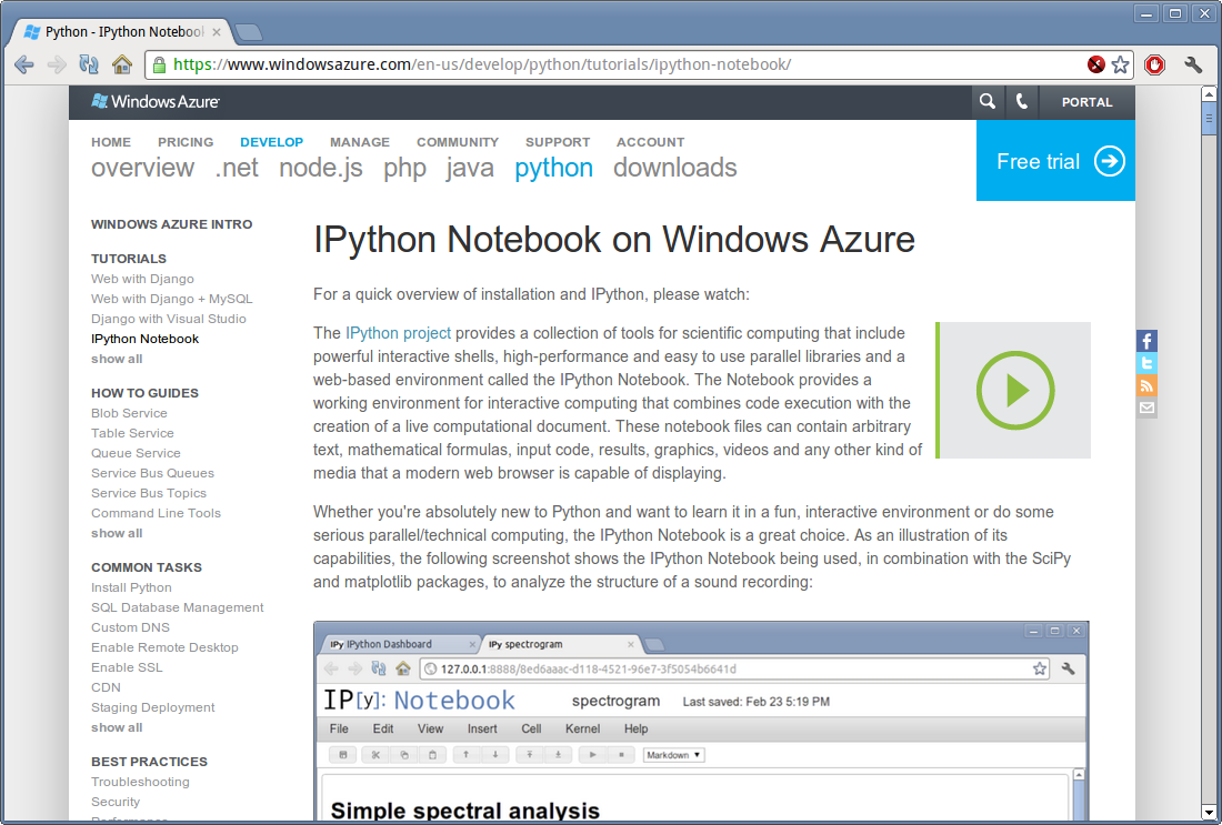
- Microsoft: WinHPC support, Visual Studio integration, Azure
- DoD/DRC Inc: 2011/12 (thanks to Jose Unpingco and Chris Keees).
- Indirect: NIH via NiPy grant, NSF via Sage grant.
- Google: summer of code 2005, 2010.
- Tech-X Corp., Boulder, CO: Parallel/notebook (previous versions)
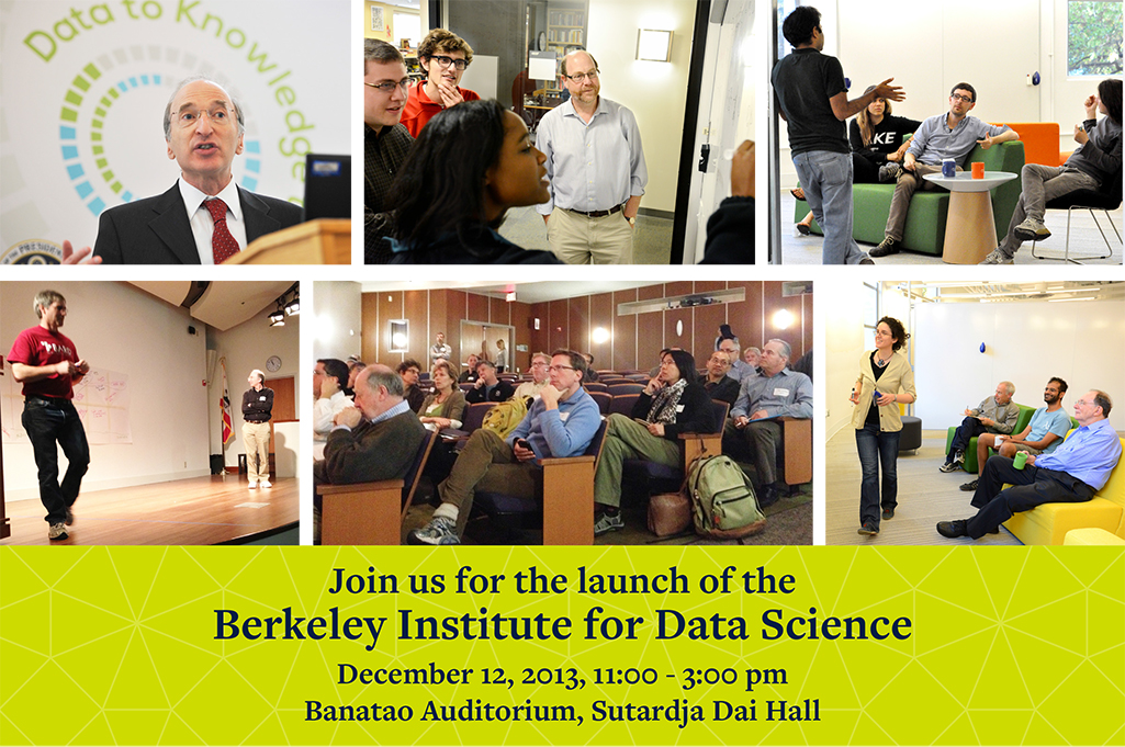
A new $37.8M initiative in Data Science
- Moore/Sloan Foundations, 5 year support for UC Berkeley, U. Washington, NYU.
- Open source scientific computing tools will be central to this effort.
- We're hiring: Executive Director (now), Data Science Fellows (soon).