Lien vers l'article de Jaddo : http://www.jaddo.fr/2016/06/19/et-mes-fesses-elles-sont-roses-mes-fesses/.
L'exemple de Jaddo
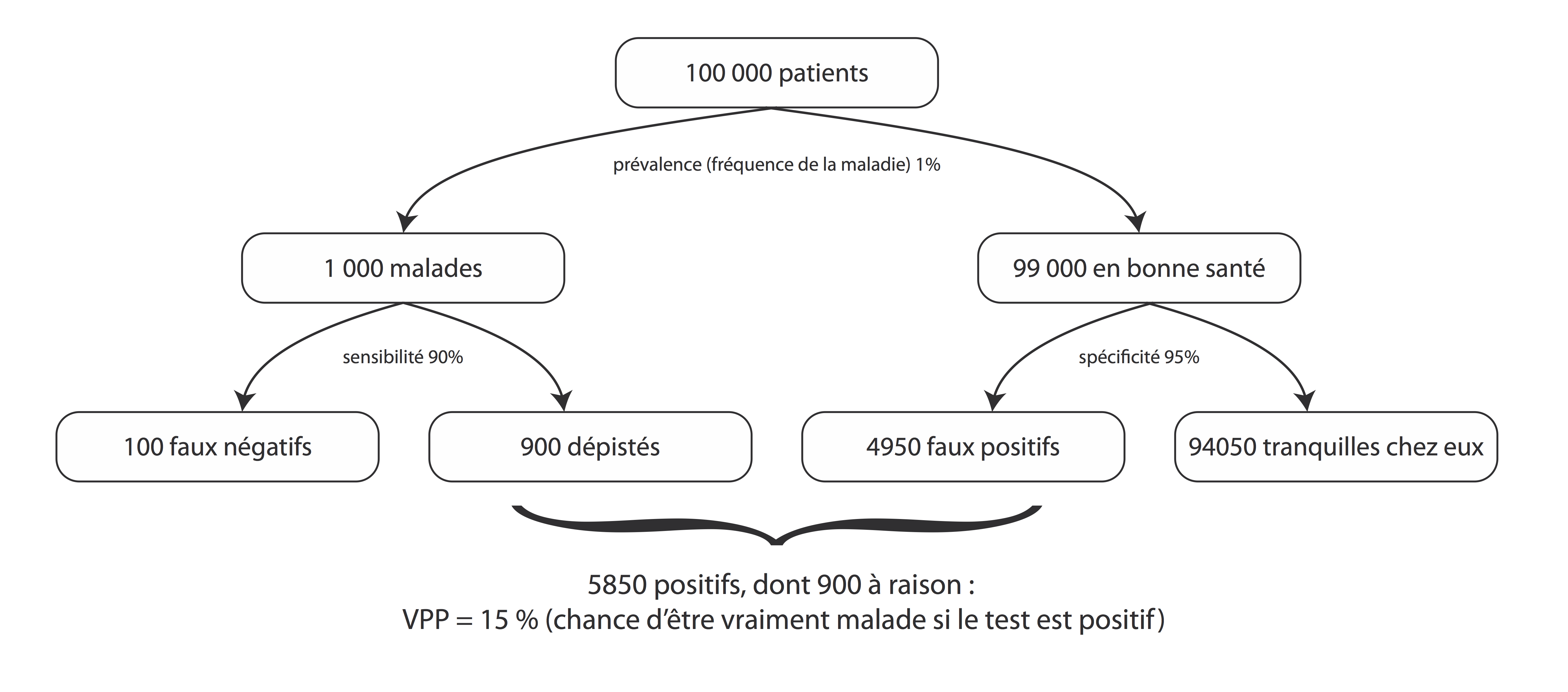
La probabilité qu’a l’examen de bien trouver l’anomalie s’il y en a une s’appelle la sensibilité.
La probabilité qu’a l’examen d’être normal quand il n’y a pas d’anomalie s’appelle la spécificité.
Valeurs d'exemple :
- sensibilité : 90 %
- spécificité : 95 %
In [3]:
n = 100000
sensi = 0.90
speci = 0.95
preva = 0.01
sick = n * preva
healthy = n - sick
true_pos = sick * sensi
false_neg = sick * (1 - sensi)
true_neg = healthy * speci
false_pos = healthy * (1 - speci)
true_pos, false_neg, true_neg, false_pos
Out[3]:
(900.0, 99.99999999999997, 94050.0, 4950.000000000005)
La probabilité que vous ayez vraiment une anomalie si le test dit qu’il y en a une, ça s’appelle la valeur prédictive positive. (VPP pour les intimes).
La probabilité que vous n’ayez pas d’anomalie si le test dit que tout va bien, ça s’appelle la valeur prédictive négative (VPN).
In [4]:
def compute_vpp_vpn(preva, sensi, speci):
    n = 100000
    sick = n * preva
    healthy = n - sick
    true_pos = sick * sensi
    false_neg = sick * (1 - sensi)
    true_neg = healthy * speci
    false_pos = healthy * (1 - speci)
    vpp = true_pos / (true_pos + false_pos)
    vpn = true_neg / (true_neg + false_neg)
    return vpp, vpn
In [5]:
vpp, vpn = compute_vpp_vpn(preva, sensi, speci)
vpp, vpn
Out[5]:
(0.15384615384615372, 0.9989378651088688)
Interactif
In [6]:
from ipywidgets import interact, fixed
In [7]:
@interact
def crunch_numbers(sensi=(0, 1., 0.01), speci=(0, 1., 0.01), preva=(0, 1., 0.01)):
    """Calcul et arbre des différents chiffres."""
    n = 100000
    sick = n * preva
    healthy = n - sick
    true_pos = sick * sensi
    false_neg = sick * (1 - sensi)
    true_neg = healthy * speci
    false_pos = healthy * (1 - speci)
    vpp = true_pos / (true_pos + false_pos)
    vpn = true_neg / (true_neg + false_neg)
    print('sick: {:n}, healthy: {:n}'.format(sick, healthy))
    print('true_positives: {:n}, false_negatives: {:n}'.format(true_pos, false_neg))
    print('true_negatives: {:n}, false_positives: {:n}'.format(true_neg, false_pos))
    print('vpp: {:.2f}, vpn: {:.2f}'.format(vpp, vpn))
Un graphique en 2d
In [8]:
import matplotlib.pyplot as plt
import numpy as np
%matplotlib inline
In [9]:
%config InlineBackend.figure_format = 'retina'
In [10]:
plt.rcParams['figure.dpi'] = 100
In [11]:
sensi_grid = np.linspace(0.01, 1, num=50)[:, np.newaxis]
speci_grid = np.linspace(0.01, 1, num=100)[np.newaxis, :]
In [12]:
n = 100000
sick = n * preva
healthy = n - sick
true_pos = sick * sensi_grid
false_neg = sick * (1 - sensi_grid)
true_neg = healthy * speci_grid
false_pos = healthy * (1 - speci_grid)
vpp = true_pos / (true_pos + false_pos)
vpn = true_neg / (true_neg + false_neg)
In [13]:
plt.imshow(vpp.T, aspect='auto', origin='lower',
           extent=(sensi_grid.min(), sensi_grid.max(), speci_grid.min(), speci_grid.max()))
plt.colorbar()
plt.xlabel('spécificité')
plt.ylabel('sensibilité')
Out[13]:
<matplotlib.text.Text at 0x110a5b668>

On le rend interactif :
In [14]:
@interact
def vpp_vpn_plot(preva=(0.01, 1, 0.01)):
    n = 100000
    sick = n * preva
    healthy = n - sick
    true_pos = sick * sensi_grid
    false_neg = sick * (1 - sensi_grid)
    true_neg = healthy * speci_grid
    false_pos = healthy * (1 - speci_grid)
    vpp = true_pos / (true_pos + false_pos)
    vpn = true_neg / (true_neg + false_neg)

    plt.figure(figsize=(10, 5))
    plt.subplot(121)
    plt.imshow(vpp.T, aspect='auto', origin='lower',
           extent=(sensi_grid.min(), sensi_grid.max(), speci_grid.min(), speci_grid.max()))
    plt.colorbar()
    plt.xlabel('spécificité')
    plt.ylabel('sensibilité')
    plt.title('VPP')

    plt.subplot(122)
    plt.imshow(vpn.T, aspect='auto', origin='lower',
           extent=(sensi_grid.min(), sensi_grid.max(), speci_grid.min(), speci_grid.max()))
    plt.colorbar()
    plt.xlabel('spécificité')
    plt.ylabel('sensibilité')
    plt.title('VPN')

    plt.tight_layout()
    plt.show()
Reproduction de l'illustration de Jaddo
In [16]:
@interact
def draw_figure(sensi = (0.01, 1., 0.01), speci = (0.01, 1., 0.01), preva = (0.01, 1., 0.01)):

    fig = plt.figure(figsize=(10, 5))
    ax = fig.add_subplot(111, autoscale_on=False, xlim=(-15, 20), ylim=(-5, 1))

    # plotting options
    bbox_dict = dict(boxstyle="round",
                                fc=(1.0, 0.7, 0.7),
                                ec=(1., .5, .5))
    size = 12.5
    dx = 7.5
    dy = 2
    # test data

    sick = n * preva
    healthy = n - sick
    true_pos = sick * sensi
    false_neg = sick * (1 - sensi)
    true_neg = healthy * speci
    false_pos = healthy * (1 - speci)
    true_pos, false_neg, true_neg, false_pos

    ann = ax.annotate('{:n} patients (prévalence {:.1f} %)'.format(n, preva * 100),
                      xy=(0., 0), xycoords='data', ha='center',
                      size=size,
                      bbox=bbox_dict)

    ax.annotate('{:n} malades'.format(sick),
                      xy=(-dx, -dy), xycoords='data', ha='center',
                      size=size,
                      bbox=bbox_dict)

    ax.annotate('{:n} en bonne santé'.format(healthy),
                      xy=(dx, -dy), xycoords='data', ha='center',
                      size=size,
                      bbox=bbox_dict)


    ax.annotate('{:n} faux négatifs'.format(false_neg),
                      xy=(-2*dx, -2*dy), xycoords='data', ha='center',
                      size=size,
                      bbox=bbox_dict)

    ax.annotate('{:n} dépistés'.format(true_pos),
                      xy=(-0.5*dx, -2*dy), xycoords='data', ha='center',
                      size=size,
                      bbox=bbox_dict)

    ax.annotate('{:n} faux positifs'.format(false_pos),
                      xy=(0.5*dx, -2*dy), xycoords='data', ha='center',
                      size=size,
                      bbox=bbox_dict)

    ax.annotate('{:n} tranquilles chez eux'.format(true_neg),
                      xy=(2*dx, -2*dy), xycoords='data', ha='center',
                      size=size,
                      bbox=bbox_dict)

    arrow_width=0.1
    arrow_hl = 1.5
    plt.arrow(0, 0, dx,  -dy*0.8, length_includes_head=True, width=arrow_width, head_length=arrow_hl, fc='k')
    plt.arrow(0, 0, -dx, -dy*0.8, length_includes_head=True, width=arrow_width, head_length=arrow_hl, fc='k')

    plt.arrow(dx, -dy, dx,  -dy*0.8, length_includes_head=True, width=arrow_width, head_length=arrow_hl, fc='k')
    plt.arrow(dx, -dy, -0.5*dx, -dy*0.8, length_includes_head=True, width=arrow_width, head_length=arrow_hl, fc='k')

    plt.arrow(-dx, -dy, -dx,  -dy*0.8, length_includes_head=True, width=arrow_width, head_length=arrow_hl, fc='k')
    plt.arrow(-dx, -dy, 0.5*dx, -dy*0.8, length_includes_head=True, width=arrow_width, head_length=arrow_hl, fc='k')
    vpp, vpn = compute_vpp_vpn(preva, sensi, speci)
    plt.text(0, 0.5, "propriétés du test : \nsensibilité {:.0f} %, spécificité {:.0f} %\nVPP : {:.0f} %, VPN : {:.0f} %".format(sensi * 100, speci * 100, vpp*100, vpn*100), ha='center')
    plt.axis('off')
    plt.show()
L'exemple de Jaddo
In [17]:
draw_figure(preva=.01, sensi=.90, speci=.95)

PSA valeur basse spécificité
In [18]:
draw_figure(preva=.02, sensi=.75, speci=.65)

PSA valeur haute spécificité
In [19]:
draw_figure(preva=.02, sensi=.75, speci=.85)

Colorectal
In [20]:
draw_figure(preva=.035, sensi=.60, speci=.96)

In [21]:
draw_figure(preva=.005, sensi=.60, speci=.96)

Le deuxième test : de confirmation
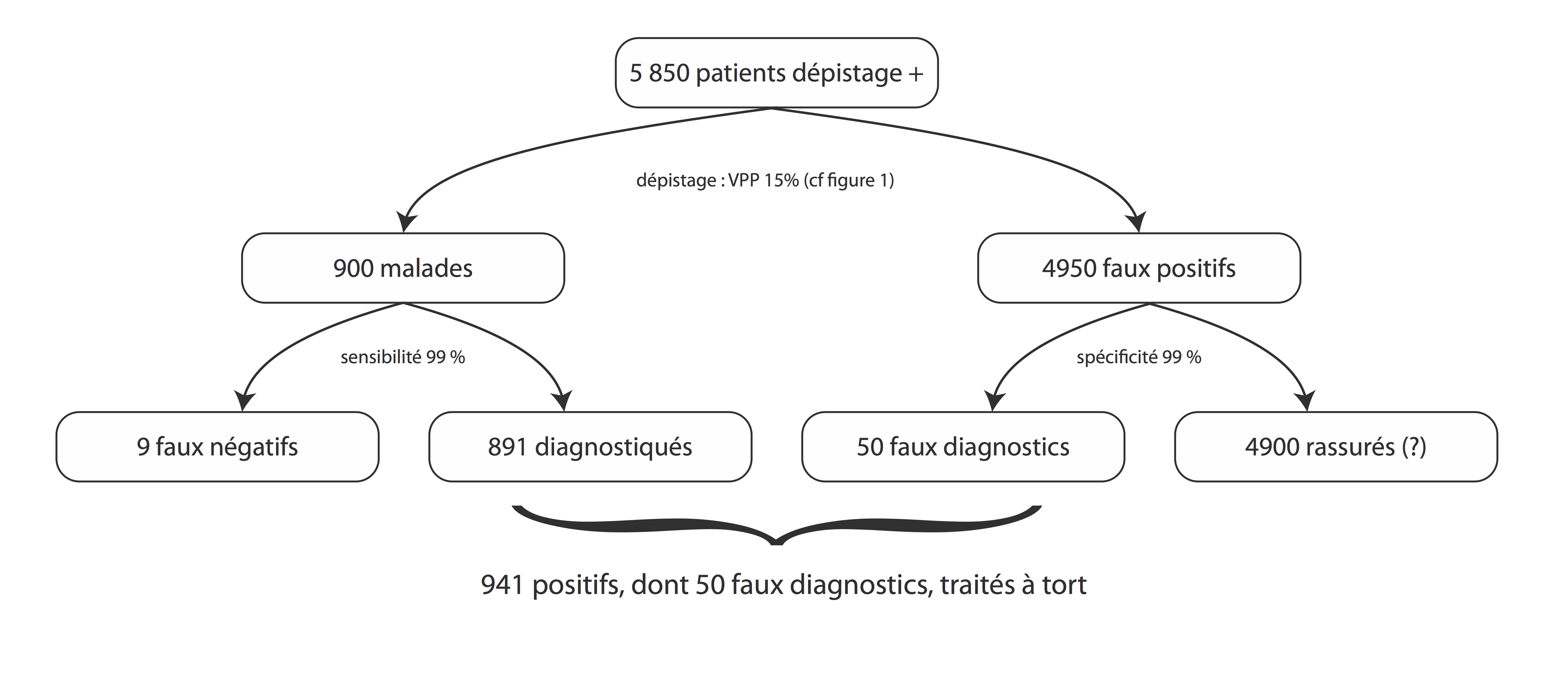
In [22]:
@interact
def draw_figure_confirmation(sensi = (0.01, 1., 0.01), speci = (0.01, 1., 0.01), true_pos_depi=fixed(900), false_pos_depi=fixed(4950)):

    fig = plt.figure(figsize=(10, 5))
    ax = fig.add_subplot(111, autoscale_on=False, xlim=(-15, 20), ylim=(-5, 1))

    # plotting options
    bbox_dict = dict(boxstyle="round",
                                fc=(0.1, 0.8, 0.1),
                                ec=(0., 0., 0.))
    size = 12
    dx = 7.5
    dy = 2

    # test data
    n = true_pos_depi + false_pos_depi
    sick = true_pos_depi
    healthy = n - sick
    true_pos = sick * sensi
    false_neg = sick * (1 - sensi)
    true_neg = healthy * speci
    false_pos = healthy * (1 - speci)
    true_pos, false_neg, true_neg, false_pos

    ann = ax.annotate('{:n} patients dépistage positif)'.format(n, preva * 100),
                      xy=(0., 0), xycoords='data', ha='center',
                      size=size,
                      bbox=bbox_dict)

    ax.annotate('{:n} malades'.format(sick),
                      xy=(-dx, -dy), xycoords='data', ha='center',
                      size=size,
                      bbox=bbox_dict)

    ax.annotate('{:n} en bonne santé'.format(healthy),
                      xy=(dx, -dy), xycoords='data', ha='center',
                      size=size,
                      bbox=bbox_dict)


    ax.annotate('{:n} faux négatifs'.format(false_neg),
                      xy=(-2*dx, -2*dy), xycoords='data', ha='center',
                      size=size,
                      bbox=bbox_dict)

    ax.annotate('{:n} diagnostiqués'.format(true_pos),
                      xy=(-0.6*dx, -2*dy), xycoords='data', ha='center',
                      size=size,
                      bbox=bbox_dict)

    ax.annotate('{:.0f} faux diagnostics'.format(false_pos),
                      xy=(0.5*dx, -2*dy), xycoords='data', ha='center',
                      size=size,
                      bbox=bbox_dict)

    ax.annotate('{:.0f} rassurés (?)'.format(true_neg),
                      xy=(2*dx, -2*dy), xycoords='data', ha='center',
                      size=size,
                      bbox=bbox_dict)

    arrow_width=0.1
    arrow_hl = 1.5
    plt.arrow(0, 0, dx,  -dy*0.8, length_includes_head=True, width=arrow_width, head_length=arrow_hl, fc='k')
    plt.arrow(0, 0, -dx, -dy*0.8, length_includes_head=True, width=arrow_width, head_length=arrow_hl, fc='k')

    plt.arrow(dx, -dy, dx,  -dy*0.8, length_includes_head=True, width=arrow_width, head_length=arrow_hl, fc='k')
    plt.arrow(dx, -dy, -0.5*dx, -dy*0.8, length_includes_head=True, width=arrow_width, head_length=arrow_hl, fc='k')

    plt.arrow(-dx, -dy, -dx,  -dy*0.8, length_includes_head=True, width=arrow_width, head_length=arrow_hl, fc='k')
    plt.arrow(-dx, -dy, 0.5*dx, -dy*0.8, length_includes_head=True, width=arrow_width, head_length=arrow_hl, fc='k')
    vpp, vpn = compute_vpp_vpn(preva, sensi, speci)
    plt.text(0, 0.5, "propriétés du test de confirmation : \nsensibilité {:.0f} %, spécificité {:.0f} %\nVPP : {:.0f} %, VPN : {:.0f} %".format(sensi * 100, speci * 100, vpp*100, vpn*100), ha='center')
    plt.axis('off')
    plt.show()
In [23]:
draw_figure_confirmation(sensi=0.99, speci=0.99, true_pos_depi=900, false_pos_depi=4950)

sankey ?
In [31]:
from matplotlib.sankey import Sankey
In [59]:
fig, ax = plt.subplots()
sankey = Sankey(ax=ax, scale=0.0015, head_angle=140, margin=13)
sankey.add(flows=[100000, -99000, -1000],
       labels=['patients', 'sains', 'malades'],
          orientations=[0, 0, 0],
          rotation=-90,
          trunklength=10.,
          pathlengths=[0, 10, 10],
          )
sankey.finish()
Out[59]:
[Bunch(patch=Poly((75, 4.75) ...), flows=[100000 -99000  -1000], angles=[-1.0, -1.0, -1.0], tips=[[  1.38065257e-15  -2.25477676e+01]
  [  7.50000000e-01  -4.17857090e+01]
  [ -7.42500000e+01  -2.47838968e+01]], text=Text(0,0,''), texts=[<matplotlib.text.Text object at 0x11ac6e2b0>, <matplotlib.text.Text object at 0x11ac6e278>, <matplotlib.text.Text object at 0x11ac6e6d8>])]

In [24]:
fig = plt.figure(figsize=(8, 12))
ax = fig.add_subplot(1, 1, 1, xticks=[], yticks=[],
                     title="Statistics from the 2nd edition of\nfrom Audio Signal Processing for Music Applications by Stanford University\nand Universitat Pompeu Fabra of Barcelona on Coursera (Jan. 2016)")
learners = [14460, 9720, 7047, 3059, 2149, 351]
labels = ["Total learners joined", "Learners that visited the course", "Learners that watched a lecture",
         "Learners that browsed the forums", "Learners that submitted an exercise",
          "Learners that obtained a grade >70%\n(got a Statement of Accomplishment)"]
colors = ["#FF0000", "#FF4000", "#FF8000", "#FFBF00", "#FFFF00"]

sankey = Sankey(ax=ax, scale=0.0015, offset=0.3)
for input_learner, output_learner, label, prior, color in zip(learners[:-1], learners[1:],
                                                              labels, [None, 0, 1, 2, 3],
                                                             colors):
    if prior != 3:
        sankey.add(flows=[input_learner, -output_learner, output_learner - input_learner],
               orientations=[0, 0, 1],
               patchlabel=label,
               labels=['', None, 'quit'],
              prior=prior,
              connect=(1, 0),
               pathlengths=[0, 0, 2],
              trunklength=10.,
              rotation=-90,
                  facecolor=color)
    else:
        sankey.add(flows=[input_learner, -output_learner, output_learner - input_learner],
               orientations=[0, 0, 1],
               patchlabel=label,
               labels=['', labels[-1], 'quit'],
              prior=prior,
              connect=(1, 0),
               pathlengths=[0, 0, 10],
              trunklength=10.,
              rotation=-90,
                  facecolor=color)
diagrams = sankey.finish()
for diagram in diagrams:
    diagram.text.set_fontweight('bold')
    diagram.text.set_fontsize('10')
    for text in diagram.texts:
        text.set_fontsize('10')
ylim = plt.ylim()
plt.ylim(ylim[0]*1.05, ylim[1])
Out[24]:
(-69.520770818713231, 5.1500000000000012)

In [ ]: