Dealing with Nails Outside of the SG Range of Table 12N
I've noticed that one brace assignment generated (Fall 2016) used a species (White Oak) that had a SG value (0.73) above the values in table 12N (pg 109 or 121 of 202). This is demonstrating the linearity of the nail capacities with regard to SG values.
Note: The values in Table 12N are supposed to be based on the equations in Table 12.3.1A (page 81 or 93 of 202).
from IPython.display import HTML

HTML('''<script>
code_show=true;
function code_toggle() {
 if (code_show){
 $('div.input').hide();
 } else {
 $('div.input').show();
 }
 code_show = !code_show
}
$( document ).ready(code_toggle);
</script>
<form action="javascript:code_toggle()"><input type="submit" value="Click here to toggle on/off the raw code."></form>''')
Table 12N Data
import pandas as pd
df = pd.read_csv('./Nails/Nail_table.csv')
two_by = df[df['Side Member']=='1-1/2']
brace = two_by[two_by['Common']=='16d']
brace
| Side Member | dia. | Common | Box | Sinker | 0.67 | 0.55 | 0.5 | 0.49 | 0.46 | 0.43 | 0.42 | 0.37 | 0.36 | 0.35 | |
|---|---|---|---|---|---|---|---|---|---|---|---|---|---|---|---|
| 1 | 1-1/2 | 0.162 | 16d | 40d | NaN | 184 | 154 | 141 | 138 | 131 | 122 | 120 | 106 | 104 | 101 |
sgs = list(brace.columns[5:])
SGs = [float(sg) for sg in sgs]
# print(SGs)
cap = [int(c) for c in list(brace[sgs].values[0])]
# print(cap)
from IPython.display import Latex
import numpy as np
m,b = np.polyfit(SGs,cap,1)
x = np.linspace(min(SGs), max(SGs))
y = m*x+b
x_proj = np.linspace(max(SGs),0.73)
y_proj = m*x_proj+b
x_fit = 0.73
y_fit = m*0.73+b
x_intr = 0.73
y_intr = (184-154)/(0.67-0.55)*(x_intr-0.55)+154
# print(y_intr)
Visualization
import matplotlib.pyplot as plt
%matplotlib inline
fig, ax = plt.subplots(1, 1, figsize=(8, 6))
plt.plot(SGs,cap,'ro', Label='Table 12N Values')
plt.plot(x,y, label='Linear Regression Fit')
plt.plot(x_proj,y_proj, 'b', linestyle=':',label='Linear Regression Projection')
plt.plot(x_fit,y_fit, 'bo', fillstyle='none', Label='Linear Fit Regression Projection')
plt.plot(x_intr,y_intr,'g*',fillstyle='none', Label='Linear Extrapolation Projection')

plt.xlabel('SG Values')
plt.ylabel('16d Common Nail Capacity')
plt.title('SG vs. 16d Nail Capacity for 1-1/2 Side Member (12N)\nWhite Oak (SG = 0.73) Extrapolation')
plt.legend(loc='upper left', shadow=True)
<matplotlib.legend.Legend at 0x7f5015390358>

Linear Regression
# print(y_fit)
fit = r'$$\text{Using Linear Regression}\\$$'
fit += (r'$$b = \frac{\sum_{i=1}^n x_i^2 \sum_{i=1}^n y_i  - \sum_{i=1}^n x_i'
        r' \sum_{i=1}^n x_i y_i}{n \sum_{i=1}^n x_i^2 - '
        r'\left(\sum_{i=1}^n x_i \right)^2} \\$$')
fit += (r'$$m = \frac{n \sum_{i=1}^n x_i y_i  - \sum_{i=1}^n x_i \sum_{i=1}^n'
        r' y_i}{n \sum_{i=1}^n x_i^2 - \left(\sum_{i=1}^n x_i \right)^2} \\$$')
fit += r'$$y = m\cdot x + b $$ $$\\$$ $$y= {:0.2f}\cdot{} + {:0.2f} = {:0.2f}$$'.format(m,x_fit,b,y_fit)
Latex(fit)
Linear Extrapolation
intrp = r'$$y = \frac{y_i - y_{i-1}}{x_i - x_{i-1}}(x - x_{i-1})+y_{i-1}$$ $$\\$$ '
intrp += r'$$y = \frac{184-154}{0.67-0.55}(0.73-0.55)+154 = %0.1f$$'%y_intr
Latex(r' $$\text{Using Linear Extrapolation}\\$$ '+intrp)
Alternatively - NDS Table 12.3.1A Yield Limit Equations
Using the minimum $Z$ value from the following equations.
$$Z = \frac{D l_m F_{em}}{R_d}$$$$Z = \frac{D l_s F_{es}}{R_d}$$$$Z = \frac{k_1 D l_s F_{es}}{R_d}$$$$Z = \frac{k_2 D l_m F_{em}}{\left(1+ 2 R_e \right)R_d}$$$$Z = \frac{k_3 D l_s F_{em}}{\left(2+ R_e \right)R_d }$$$$Z = \frac{D^2}{R_d}\sqrt{\frac{2 F_{em} F_{yb}}{3 \left(1+R_e \right)}}$$Where:
$\displaystyle k_1 = \frac{\sqrt{R_e + 2 R_e^2 \left(1+R_t R_t^2 \right)+R_t^2 R_e^3}-R_e\left(1+ R_t \right)}{\left(1+R_e \right)}$
$\displaystyle k_2 = -1 + \sqrt{2\left(1+R_e \right)+\frac{2 F_yb\left(1+2R_e \right)D^2}{3 F_{em} l_m^2}}$
$\displaystyle k_3 = -1 + \sqrt{\frac{2\left(1+R_e \right)}{R_e}+\frac{2 F_yb\left(2+R_e \right)D^2}{3 F_{em} l_s^2}}$
- $D$ = diameter, in. (see 12.3.7)
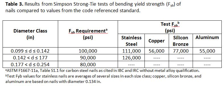
- $F_{yb}$ = dowel bending yield strength, psi (Use $\mathbf{F_{yb}}$ Requirements in Table 3 below)
- $R_d$ = reduction term (see Table 12.3.1B)
- $R_e$ = $F_{em} /F_{es}$
- $R_t$ = $l_m / s$
- $l_m$ = main member dowel bearing length, in.
- $l_s$ = side member dowel bearing length, in.
- $F_{em}$ = main member dowel bearing strength, psi (see Table 12.3.3)
- $F_{es}$ = side member dowel bearing strength, psi (see Table 12.3.3)