Exploring Accelerometer Data from OpenBCI
EEG Hacker, 2014-11-23, MIT License
Purpose
Record accelerometer data from OpenBCI V3 board during known motions. Confirm that the data matches the known motions.
Setup
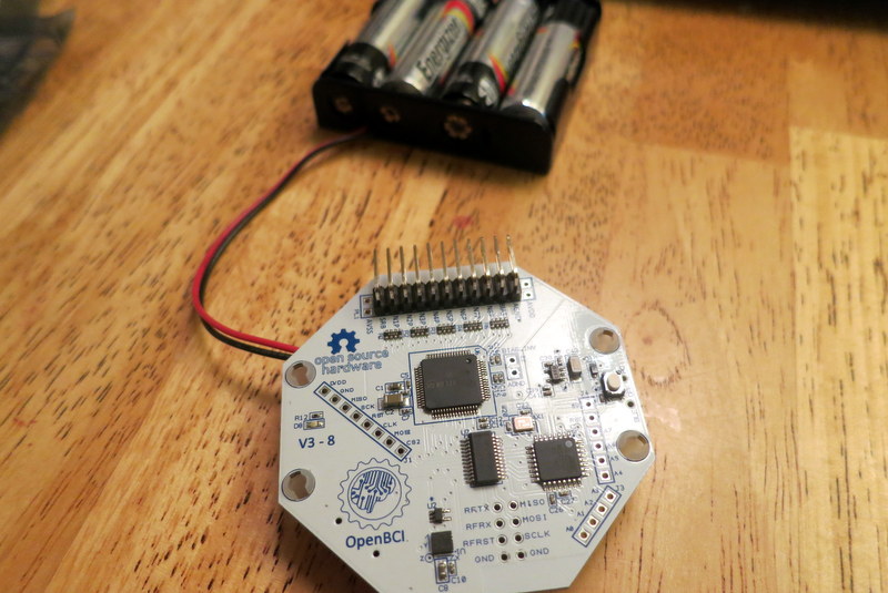
OpenBCI V3 Board (see below) with software as delivered from OpenBCI. Data was logged using the OpenBCI GUI in Processing.
Procedure
I inserted the batteries to my OpenBCI board to give it power. I started the OpenBCI GUI to begin recording data. Holding the board in my hand, I completed the following maneuvers:
- Start with board flat and level (z-axis points up)
- Roll it 90 deg to the right (x-axis points down) and 90 deg left (x-axis points up)
- Tip it nose down (y-axis points down) and nose up (y-axis points up)
- Flip it upside down (z-axis points down)
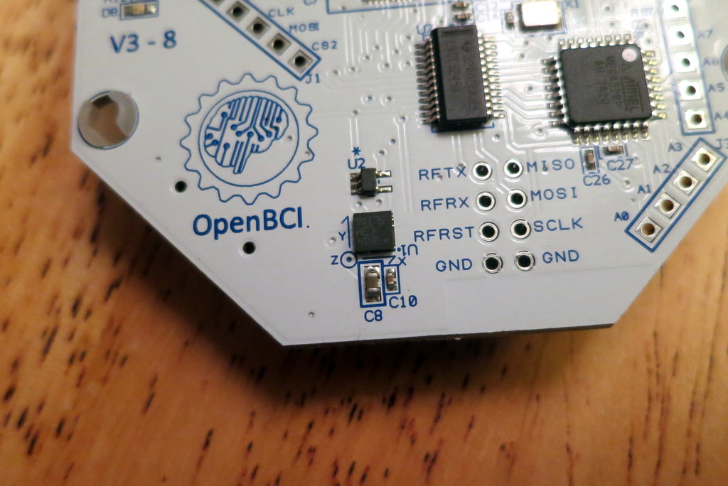
Notice the markings on the OpenBCI board that indicate the direction of the axes.
Data and Analysis Files
The 3-axis accelerometer data was saved to a text file by the Processing GUI. I analyzed the data using Python. The data and analysis files are available on my EEGHacker repo on GitHub. Be sure to unzip the ZIP file in the SavedData/ directory!
Results
The specific goals of this analysis are to confirm that the data is well behaved, that the correct axes are responding to the known motions, that the units are correct, and that the scale factors are correct.
# First, import the Python libraries that we need
%matplotlib inline
import matplotlib.pyplot as plt
import numpy as np
# Define Data to Load...be sure to UNZIP the data!!!
pname = 'SavedData/'
fname = 'OpenBCI-RAW-2014-11-23_18-54-57.txt'

# load data into numpy array
fs_Hz = 250.0        # assumed sample rate for the EEG data
data = np.loadtxt(pname + fname,
                  delimiter=',',
                  skiprows=5)

# check the packet counter for dropped packets
data_indices = data[:, 0]   # the first column is the packet index
d_indices = data_indices[2:]-data_indices[1:-1]
n_jump = np.count_nonzero((d_indices != 1) & (d_indices != -255))
print("Number of discontinuities in the packet counter: " + str(n_jump))
Number of discontinuities in the packet counter: 0
Finding: Based on the result above, we appear to have received all of the data packets that we wirelessly sent from the OpenBCI board. This is good.
# parse the data out of the values read from the text file
# eeg_data_uV = data[:, 1:(8+1)] # EEG data, microvolts
accel_data_counts = data[:, 9:(11+1)]  # note, accel data is NOT in engineering units

# convert units
unused_bits = 4 #the 4 LSB are unused?
accel_data_counts = accel_data_counts / (2**unused_bits) # strip off this extra LSB
scale_G_per_count = 0.002  # for full-scale = +/- 4G, scale is 2 mG per count
accel_data_G = scale_G_per_count*accel_data_counts # convert to G
Discussion: Based on how the default OpenBCI software configures the accelerometer, I expect the scale factor to be 2 mG per count. Furthermore, when this data was recorded, the OpenBCI GUI was simply writing the raw accelerometer data to the log file (ie, the GUI was not converting the data for me). So, in this analysis of the logged acceleration data, I thought that I would simply multiply the values in the log file by 0.002 to get my values as "G". This did not turn out to be the case.
In discussions with Joel from OpenBCI, it appears that the last four bits of the raw accelerometer values are always empty (ie, the last four bits are always equal to zero). Once I shifted the raw accelerometer values down by four bits (ie, I divided the values by 16), I seem to get the correct acceleration values. I did not notice any mention of this in the accelerometer's datasheet. Weird.
Since this data was taken, the accelerometer's scale factor and the divide-by-16 have been included in the OpenBCI GUI. Now, when the acceleration values are saved in the log file, it will have the units of "G". As a result, the "convert units" section that you see above will no longer be necessary.
# create a vector with the time of each sample
t_sec = np.arange(len(accel_data_G[:, 0])) / fs_Hz

# The accel data seems to be padded with lots of zeros.
I = np.nonzero(accel_data_G[:,0])
I=I[0]
print("Accel data exists in " + str(len(I)) +
      " of " + str(len(t_sec)) + \
      " (" + str((100*len(I))/len(t_sec)) +
      "%) of data packets");

# Only get the non-zero entries
accel_data_G = accel_data_G[I,:]
t_sec = t_sec[I]
Accel data exists in 924 of 9818 (9%) of data packets
Finding: We see that there are only acceleration values in 9% of the data packets. Why is there NOT acceleration data in every data packet? It's because the default software on the OpenBCI board is set to have the accelerometer produce accleration values only at a rate of 25Hz. Since the ADS1299 EEG chip is generating data at 250 Hz, I would have expected (25/250) = 10% of the packets to have acceleration values, not 9%. Still, this is close enough for this first exploration of the accelerometer data.
# plot each channel of accelerometer data
for Iaxis in range(3):
    plt.figure(figsize=(9.0, 2.5))
    plt.plot(t_sec,accel_data_G[:, Iaxis])
    plt.plot([t_sec[0], t_sec[-1]],[0, 0],'k--')
    plt.plot([t_sec[0], t_sec[-1]],[1.0, 1.0],'k:')
    plt.plot([t_sec[0], t_sec[-1]],[-1.0, -1.0],'k:')
    plt.xlabel("Time (sec)")
    plt.ylabel("Acceleration (G)")
    plt.title("Accelerometer Channel " + str(Iaxis))
    plt.ylim([-1.5, 1.5])

    # add annotations to show each movement
    if (Iaxis==0) :
        plt.text(1.0,0.25,"Flat and Level",
                 horizontalalignment='left',
                 backgroundcolor='w',
                 verticalalignment='center')
        plt.text(10.5,-0.8,"Roll Right",
                 horizontalalignment='right',
                 backgroundcolor='w',
                 verticalalignment='center')
        plt.text(18.5,0.8,"Roll Left",
                 horizontalalignment='left',
                 backgroundcolor='w',
                 verticalalignment='center')
    elif (Iaxis==1) :
        plt.text(20,-0.8,"Nose Down",
                 horizontalalignment='right',
                 backgroundcolor='w',
                 verticalalignment='center')
        plt.text(27,0.8,"Nose Up",
                 horizontalalignment='left',
                 backgroundcolor='w',
                 verticalalignment='center')
    elif (Iaxis==2) :
        plt.text(30.5,-0.8,"Upside Down",
                 horizontalalignment='right',
                 backgroundcolor='w',
                 verticalalignment='center')


Finding: In the graphs above, we can clearly see when I changed the orientation of the board. Excellent. Furthermore, we see positive acceleration when the axis arrow on the OpenBCI board points up and we see negative acceleration when the axis arrow on the board points down.
# compute magnitude of the acceleration vector
mag_accel_G = np.sqrt(accel_data_G[:,0]**2 +
                      accel_data_G[:,1]**2 +
                      accel_data_G[:,2]**2)
median_mag_accel_G = np.median(mag_accel_G)

#plot magnitude of acceleration
plt.figure(figsize=(9, 2.5))
plt.plot(t_sec,mag_accel_G)
plt.plot([t_sec[0], t_sec[-1]],[1.0, 1.0],'k--')
plt.xlabel("Time (sec)")
plt.ylabel("Acceleration (G)")
plt.title("Magnitude of Acceleration")
plt.ylim([0.6, 1.4])
plt.text(1,1.3,"Median = " + "{:.3f}".format(median_mag_accel_G) + "G")
plt.show()

print "Median acceleration should be near 1.0 G"
print "Median acceleration is actually " + \
       "{:.3f}".format(median_mag_accel_G) + " G"

Median acceleration should be near 1.0 G
Median acceleration is actually 1.044 G
Finding: We expect that when the board is not moving, the total acceleration should be about 1G (ie, just gravity). We see that the median acceleration is actually about 44 mG too high. Based on the datasheet for the LIS3DH accelerometer, however, it does say that we could a "typical" offset of 40 mG per axis. For a 3-axis device, this could result in sqrt(402 + 402 + 402) = 69 mG of offset. Our 44 mG is in-line with this expectation, so the result shown above is OK.
Summary and Conclusions
In this test, we found that:
- We get accelerometer data every 11th data packet (we expected every 10th)
- The accelerometer data correctly reflects the orientation of the OpenBCI board
- The acceleration values are positive value when pointing "up" and negative when pointing "down"
- The scale factor for the accelerometer is correct, within the expected offset error of the device
These are good results and I'm pleased. Now it's time to figure out something fun to do with the accelerometer!