Linear Regression
Preliminaries
- Goal
- Maximum likelihood estimates for various linear regression variants
- Materials
- Mandatory
- These lecture notes
- Optional
- Mandatory
Regression - Illustration
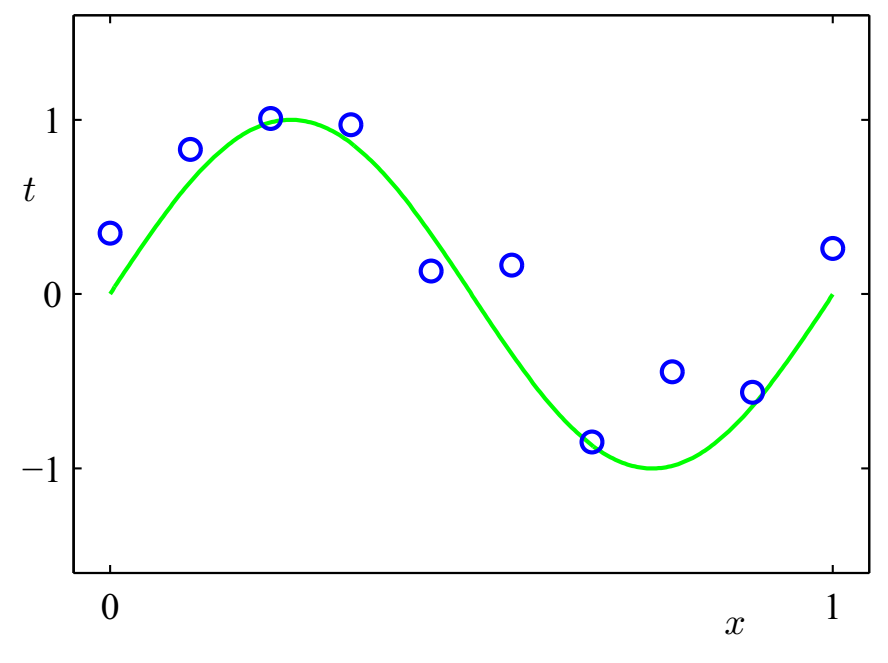
Given a set of (noisy) data measurements, find the 'best' relation between an input variable $x \in \mathbb{R}^D$ and input-dependent outcomes $y \in \mathbb{R}$
Regression vs Density Estimation
- Observe $N$ IID data pairs $D=\{(x_1,y_1),\dotsc,(x_N,y_N)\}$ with $x_n \in \mathbb{R}^D$ and $y_n \in \mathbb{R}$.
- [Q.] We could try to build a model for the data by density estimation, $p(x,y)$, but what if we are interested only in (a model for) the responses $y_n$ for given inputs $x_n$?
- [A.] We will build a model only for the conditional distribution $p(y|x)$.
- Note that, since $p(x,y)=p(y|x)\, p(x)$, this is a building block for the joint data density.
- In a sense, this is density modeling with the assumption that $x$ is drawn from a uniform distribution.
- Next, we discuss model (1) specification, (2) ML estimation and (3) prediction for the linear regression model.
1. Model Specification for Linear Regression
In a regression model, we try to 'explain the data' by a purely deterministic term $f(x,w)$, plus a purely random term $\epsilon_n$ for 'unexplained noise',
$$ y_n = f(x_n,w) + \epsilon_n $$
- In linear regression, we assume that
- In ordinary linear regression, the noise process $\epsilon_n$ is zero-mean Gaussian with constant variance $\sigma^2$, i.e.
or equivalently, the likelihood model is $$ p(y_n|\,x_n,w) = \mathcal{N}(y_n|\,w^T x_n,\sigma^2) \,. $$
- For full Bayesian learning we should also choose a prior $p(w)$; In ML estimation, the prior $p(w)$ is uniformly distributed (so it can be ignored).
2. ML Estimation for Linear Regression Model
- Let's work out the log-likelihood for multiple observations
where we defined $N\times 1$ vector $y = \left(y_1 ,y_2 , \ldots ,y_N \right)^T$ and $(N\times D)$-dim matrix $\mathbf{X} = \left( x_1 ,x_2 , \ldots ,x_n \right)^T$.
- Set the derivative $\nabla_{w} \log p(D|w) = \frac{1}{\sigma^2} \mathbf{X}^T(y-\mathbf{X} w)$ to zero for
the maximum likelihood estimate $$\begin{equation*} \boxed{\hat w_{\text{ML}} = (\mathbf{X}^T \mathbf{X})^{-1} \mathbf{X}^T y} \end{equation*}$$
- The matrix $\mathbf{X}^\dagger \equiv (\mathbf{X}^T \mathbf{X})^{-1}\mathbf{X}^T$ is also known as the Moore-Penrose pseudo-inverse (which is sort-of-an-inverse for non-square matrices).
- Note that size ($N\times D$) of the data matrix $\mathbf{X}$ grows with number of observations, but the size ($D\times D$) of $\mathbf{X}^T\mathbf{X}$ is independent of training data set.
3. Prediction of New Data Points
- Now, we want to apply the trained model. New data points can be predicted by
- Note that the expected value of a predicted new data point
can also be expressed as a linear combination of the observed data points
$$y = \left( {y_1 ,y_1 , \ldots ,y_N } \right)^T \,.$$Deterministic Least-Squares Regression
- (You may say that) we don't need to work with probabilistic models. E.g., there's also the deterministic least-squares solution: minimize sum of squared errors,
- Setting the gradient
$ \frac{\partial \left( {y - \mathbf{X}w } \right)^T \left( {y - \mathbf{X}w } \right)}{\partial w} = -2 \mathbf{X}^T \left(y - \mathbf{X} w \right) $ to zero yields the normal equations $\mathbf{X}^T\mathbf{X} \hat w_{\text{LS}} = \mathbf{X}^T y$ and consequently $$ \boxed{\hat w_{\text{LS}} = (\mathbf{X}^T \mathbf{X})^{-1} \mathbf{X}^T y} $$ which is the same answer as we got for the maximum likelihood weights $\hat w_{\text{ML}}$.
- $\Rightarrow$ Least-squares regression ($\hat w_{\text{LS}}$) corresponds to (probabilistic) maximum likelihood ($\hat w_{\text{ML}}$) if
- IID samples (determines how errors are combined), and
- Noise $\epsilon_n \sim \mathcal{N}(0,\,\sigma^2)$ is Gaussian (determines error metric)
Probabilistic vs. Deterministic Approach
- The (deterministic) least-squares approach assumed IID Gaussian distributed data, but these assumptions are not obvious from looking at the least-squares (LS) criterion.
- If the data were better modeled by non-Gaussian assumptions (or not IID), then LS might not be appropriate.
- The probabilistic approach makes all these issues completely transparent by focusing on the model specification rather than the error criterion.
- Next, we will show this by two examples: (1) samples not identically distributed, and (2) few data points.
Not Identically Distributed Data
- What if we assume that the variance of the measurement error varies with the sampling index, $\epsilon_n \sim \mathcal{N}(0,\sigma_n^2)$?
- Let's make the log-likelihood again (use $\Lambda \triangleq \mathrm{diag}[1/\sigma_n^2]$):
- Set derivative $\partial \mathrm{L(w)} / \partial w = -\mathbf{X}^T\Lambda (y-\mathbf{X} w)$
to zero to get the normal equations $\mathbf{X}^T \Lambda \mathbf{X} \hat{w}_{\text{WLS}} = \mathbf{X}^T \Lambda y$ and consequently $$ \boxed{\hat{w}_{\text{WLS}} = \left(\mathbf{X}^T \Lambda \mathbf{X}\right)^{-1} \mathbf{X}^T \Lambda y}$$
- This is also called the Weighted Least Squares (WLS) solution. (Note that we just stumbled upon it, the crucial aspect is appropriate model specification!)
- Note also that the dimension of $\Lambda$ grows with the number of data points. In general, models for which the number of parameters grow as the number of observations increase are called non-parametric models.
CODE EXAMPLE
We'll compare the Least Squares and Weighted Least Squares solutions for a simple linear regression model with input-dependent noise:
$$\begin{align*} x &\sim \text{Unif}[0,1]\\ y|x &\sim \mathcal{N}(f(x), v(x))\\ f(x) &= 5x - 2\\ v(x) &= 10e^{2x^2}-9.5\\ \mathcal{D} &= \{(x_1,y_1),\ldots,(x_N,y_N)\} \end{align*}$$using PyPlot, LinearAlgebra
# Model specification: y|x ~ 𝒩(f(x), v(x))
f(x) = 5*x .- 2
v(x) = 10*exp.(2*x.^2) .- 9.5 # input dependent noise variance
x_test = [0.0, 1.0]
plot(x_test, f(x_test), "k--") # plot f(x)
# Generate N samples (x,y), where x ~ Unif[0,1]
N = 50
x = rand(N)
y = f(x) + sqrt.(v(x)) .* randn(N)
plot(x, y, "kx"); xlabel("x"); ylabel("y") # Plot samples
# Add constant to input so we can estimate both the offset and the slope
_x = [x ones(N)]
_x_test = hcat(x_test, ones(2))
# LS regression
w_ls = pinv(_x) * y
plot(x_test, _x_test*w_ls, "b-") # plot LS solution
# Weighted LS regression
W = Diagonal(1 ./ v(x)) # weight matrix
w_wls = inv(_x'*W*_x) * _x' * W * y
plot(x_test, _x_test*w_wls, "r-") # plot WLS solution
ylim([-5,8]); legend(["f(x)", "D", "LS linear regr.", "WLS linear regr."],loc=2);

Too Few Training Samples
- If we have fewer training samples than input dimensions, $\mathbf{X}^T\mathbf{X}$ will not be invertible. (Why?)
- As a general recipe, in case of (expected) problems, go back to full Bayesian! Do proper model specification, Bayesian inference etc. Let's do this next.
- Model specification. Let's try a Gaussian prior for $w$ (why is this reasonable?)
- Learning. Let's do Bayesian inference,
- Done! The posterior $p(w|D)$ specifies all we know about $w$ after seeing the data.
Too Few Training Samples, cont'd: the MAP estimate
- As discussed, for practical purposes, you often want a point estimate for $w$, rather than a posterior distribution.
- For instance, let's take a Maximum A Posteriori (MAP) estimate. Set derivative
to zero, yielding $$ \boxed{ \hat{w}_{\text{MAP}} = \left( \mathbf{X}^T\mathbf{X} + \frac{\sigma^2}{\varepsilon} I \right)^{-1}\mathbf{X}^T y } $$
- Note that, in contrast to $\mathbf{X}^T\mathbf{X}$, the matrix $\left( \mathbf{X}^T\mathbf{X} + (\sigma^2 / \varepsilon) I \right)$ is always invertible! (Why?)
- Note also that $\hat{w}_{\text{LS}}$ is retrieved by letting $\varepsilon \rightarrow \infty$. Does that make sense?
Adaptive Linear Regression
- What if the data arrives one point at a time?
- Two standard adaptive linear regression approaches: RLS and LMS. Here we shortly recap the LMS approach.
- Least Mean Squares (LMS) is gradient-descent on a 'local-in-time' approximation of the square-error cost function.
- Define the cost-of-current-sample as
and track the optimum by gradient descent (at each sample index $n$): $$\begin{equation*} w_{n+1} = w_n - \eta \, \left. \frac{\partial E_n}{\partial w} \right|_{w_n} \end{equation*}$$ which leads to the LMS update: $$ \boxed{ w_{n+1} = w_n + \eta \, (y_n - w_n^T x_n) x_n } $$
- (OPTIONAL) This is not a probabilistic modelling derivation. Is there also a Bayesian treatment of LMS? Sure, e.g., have a look at G. Deng et al., A model-based approach for the development of LMS algorithms', ISCAS-05 symposium, 2005.
open("../../styles/aipstyle.html") do f
    display("text/html", read(f, String))
end