Solving $ A x = b $ via LU factorization and triangular solves
In this notebook, you will implement an LU factorization, solve a system with a unit lower triangular matrix, and solve a system with an upper triangular matrix. This notebook culminates in a routine that combines these three steps into a routine that solves $ A x = b $.
Be sure to make a copy!!!!
Preliminaries
Here is a list of laff routines that you might want to use in this notebook:
-
laff.dots( x, y, alpha )$\alpha := x^T y + \alpha$ -
laff.invscal( alpha, x )$x := x / \alpha$ (See note below) -
laff.axpy( alpha, x, y )$y := \alpha x + y$ -
laff.ger( alpha, x, y, A )$A := \alpha x y^T + A$
laff.invscal( alpha, x) was added after the course started. If you're having problems with git and are manually downloading the notebooks, check the wiki page for notebooks for help on getting updated laff routines.
First, let's create a matrix $ A $ and right-hand side $ b $
import numpy as np
import laff
import flame

# Applying the LU Factorization to a matrix is the process of
# computing a unit lower triangular matrix, L, and upper
# triangular matrix, U, such that A = L U.  To avoid nasty fractions
# in these caclulations, we create our matrix A from two matrices, L and U,
# whose elements we know to be integer valued.

L = np.matrix( ' 1, 0, 0. 0;\
                -2, 1, 0, 0;\
                 1,-3, 1, 0;\
                 2, 3,-1, 1' )

U = np.matrix( ' 2,-1, 3,-2;\
                 0,-2, 1,-1;\
                 0, 0, 1, 2;\
                 0, 0, 0, 3' )

A = L * U

print( 'A = ' )
print( A )

# create a solution vector x

x = np.matrix( '-1;\
                 2;\
                 1;\
                -2' )

# store the original value of x

xold = np.matrix( np.copy( x ) )

# create a solution vector b so that A x = b

b = A * x
print( 'b = ' )
print( b )

# Much later, we are also going to solve A x = y.  Here we create that y:
x2 = np.matrix( '1;\
                 2;\
                 -2;\
                 1' )
y = A * x2
print( 'y = ' )
print( y )
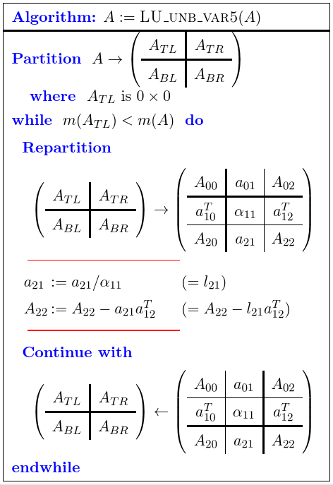
Implement the LU factorization routine from 6.3.1
Here is the algorithm:
Important: if you make a mistake, rerun ALL cells above the cell in which you were working before you rerun the one in which you are working.
Create the routine
LU_unb_var5( A )
with the Spark webpage for the algorithm given above.
# Insert code here
Test the routine
Important: if you make a mistake, rerun ALL cells above the cell in which you were working before you rerun the one in which you are working.
# recreate matrix A
A = L * U

# recreate the right-hand side
b = A * xold

# apply Gaussian elimination to matrix A
LU_unb_var5( A )
Compare the overwritten matrix, $ A $, to the original matrices, $ L $ and $ U $. The upper triangular part of $ A $ should equal $ U $ and the strictly lower triangular part of $ A $ should equal the strictly lower triangular part of $ L $.
Important: if you make a mistake, rerun ALL cells above the cell in which you were working before you rerun the one in which you are working.
print( 'A after factorization' )
print( A )
print( 'Original L' )
print( L )
print( 'Original U' )
print( U )
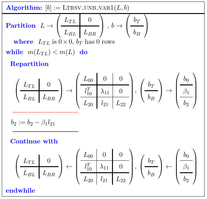
Implement the routine Ltrsv_unb_var1 from 6.3.2
(if you have not yet visited Unit 6.3.2, do so now!)
Here is the algorithm:
Important: if you make a mistake, rerun ALL cells above the cell in which you were working before you rerun the one in which you are working.
Create the routine
Ltrsv_unb_var1( L, b )
with the Spark webpage for the algorithm given above.
# Insert code here
Test Ltrsv_unb_var1
Take the output from LU_unb_var5, and use it to solve $ L z = b $, where $ L $ is unit lower triangular with its strictly lower triangular part stored in the strictly lower triangular part of $ A $.
Important: if you make a mistake, rerun ALL cells above the cell in which you were working before you rerun the one in which you are working.
print( A )
print( b )
Ltrsv_unb_var1( A, b )

print( 'updated b' )
print( b )
To be able to perform the back substitution before we implement the upper triangular solve routine described in 6.3.3, we do it the hard way here. This allows us to see if the LU factorization followed by the solve with the unit lower triangular system gives the correct intermediate result.
Important: if you make a mistake, rerun ALL cells above the cell in which you were working before you rerun the one in which you are working.
x[ 3 ] = b[ 3 ] / A[ 3,3 ]
x[ 2 ] = ( b[ 2 ] - A[ 2,3 ] * x[ 3 ] ) / A[ 2,2 ]
x[ 1 ] = ( b[ 1 ] - A[ 1,2 ] * x[ 2 ] - A[ 1,3 ] * x[ 3 ] ) / A[ 1,1 ]
x[ 0 ] = ( b[ 0 ] - A[ 0,1 ] * x[ 1 ] - A[ 0,2 ] * x[ 2 ]- A[ 0,3 ] * x[ 3 ] ) / A[ 0,0 ]
print( 'x = ' )
print( x )

print( 'x - xold' )
print( x - xold )
x - xold should yield a zero vector
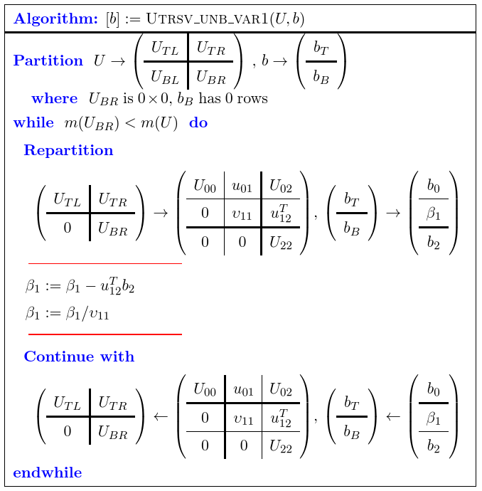
Implement the routine Utrsv_unb_var1 from 6.3.3
(if you have not yet visited Unit 6.3.3, do so now!)
Here is the algorithm:
Important: if you make a mistake, rerun ALL cells above the cell in which you were working before you rerun the one in which you are working.
Create the routine
Utrsv_unb_var1( U, b )
with the Spark webpage for the algorithm given above.
Hint: Implement $ \beta_1 := \beta - u_{12}^T b_2 $ as laff.dots( -u12t, b2, beta1 )
# Insert code here
Test Utrsv_unb_var1
Take the output from LU_unb_var5 and Ltrsv_unb_var1 and use it to solve $ U x = b $, where $ U $ is upper triangular and stored in the upper triangular part of $ A $.
Important: if you make a mistake, rerun ALL cells above the cell in which you were working before you rerun the one in which you are working.
# just to be sure, let's start over.  We'll recreate A, x, and b, run all the routines, and
# then compare the updated b to the original vector x.

A = L * U
b = A * x

LU_unb_var5( A )
Ltrsv_unb_var1( A, b )
Utrsv_unb_var1( A, b )

print( 'updated b' )
print( b )
print( 'original x' )
print( x )
print( 'b - x' )
print( b - x )
In theory, b - x should yield a zero vector...
Implement the routine Solve from 6.3.4
(if you have not yet visited Unit 6.3.4, do so now!)
This time, we do NOT use Spark! What we need to do is write a routine that, when given a matrix $ A $ and right-hand side vector $ b $, solves $ A x = b $, overwriting $ A $ with the LU factorization and overwriting $ b $ with the solution vector $ x $:
- $ A \rightarrow L U $, overwriting $ A $ with $ L $ and $ U $.
- Solve $ L z = b $, overwriting $ b $ with $ z $.
- Solve $ U x = z $, where $ z $ is stored in vector $ b $ and $ x $ overwrites $ b $.
Important: if you make a mistake, rerun ALL cells above the cell in which you were working before you rerun the one in which you are working.
Create the routine
Solve( A, b )
def Solve( A, b ):

    # insert appropriate calls to routines you have written here!
Test Solve
Important: if you make a mistake, rerun ALL cells above the cell in which you were working before you rerun the one in which you are working.
# just to be sure, let's start over.  We'll recreate A, x, and b, run all the routines, and
# then compare the updated b to the original vector x.

A = L * U
b = A * x

Solve( A, b )

print( 'updated b' )
print( b )
print( 'original x' )
print( x )
print( 'b - x' )
print( b - x )
In theory, b - x should yield a zero vector...
What if a new right-hand side comes along?
What if we are presented with a new right-hand side, call it $ y $, with which we want to solve $ A x = y $, overwriting $ y $ with the solution? (We created such a $ y $ at the top of this notebook.)
Notice that you can take the matrix $A $ that was modified by Solve and use it with Ltrsv_unb_var1 and Utrsv_unb_var1:
# insert appropriate calls here.


print( 'y = ' )
print( y )

print( 'x2 - y =' )
print( x2 - y )
x2 - y should evaluate to the zero vector.
Important: you should not refactor $ A $!!!!