Gaussian Elimination
In this notebook, we walk you through the steps that take you from applying Gauss transforms to a matrix to an algorithm that performs these steps.
Be sure to make a copy!!!!
Preliminaries
Here is a list of laff routines that you might want to use in this notebook:
-
laff.invscal( alpha, x )$x := x / \alpha$ (See note below) -
laff.axpy( alpha, x, y )$y := \alpha x + y$ -
laff.ger( alpha, x, y, A )$A := \alpha x y^T + A$
laff.invscal( alpha, x) was added after the course started. If you're having problems with git and are manually downloading the notebooks, check the wiki page for notebooks for help on getting updated laff routines.
First, let's create a matrix
import numpy as np
import laff
import flame

# Later this week, you will find out that applying Gaussian Elimination to a matrix
# is equivalent to computing a unit lower triangular matrix, L, and upper
# triangular matrix, U, such that A = L U.  Here we use that fact to create a
# matrix with which to perform Gaussian elimination that doesn't have nasty fractions.

L = np.matrix( ' 1, 0, 0. 0;\
                -2, 1, 0, 0;\
                 1,-3, 1, 0;\
                 2, 3,-1, 1' )

U = np.matrix( ' 2,-1, 3,-2;\
                 0,-2, 1,-1;\
                 0, 0, 1, 2;\
                 0, 0, 0, 3' )

A = L * U

print( 'A = ' )
print( A )

# create a solution vector x

x = np.matrix( '-1;\
                 2;\
                 1;\
                -2' )

# store the original value of x

xold = np.matrix( np.copy( x ) )

# create a solution vector b so that A x = b

b = A * x
print( 'b = ' )
print( b )
Solution via Gauss transforms
Let's use a sequence of Gauss transforms to reduce the matrix to an upper triangular matrix. We then apply the Gauss transforms to the right-hand side $ b $. Finally, we perform backsubstition. Well, actually, here we have Python do the work for us.
Step 1:
$ \left( \begin{array}{c c c c} 1 & 0 & 0 & 0 \\ -\lambda_{1,0} & 1 & 0 & 0 \\ -\lambda_{2,0} & 0 & 1 & 0 \\ -\lambda_{3,0} & 0 & 0 & 1 \end{array} \right) \left( \begin{array}{ c c c c} \alpha_{0,0} & \alpha_{0,1} & \alpha_{0,2} & \alpha_{0,3} \\ \alpha_{1,0} & \alpha_{1,1} & \alpha_{1,2} & \alpha_{1,3} \\ \alpha_{2,0} & \alpha_{2,1} & \alpha_{2,2} & \alpha_{2,3} \\ \alpha_{3,0} & \alpha_{3,1} & \alpha_{3,2} & \alpha_{3,3} \end{array} \right) \rightarrow \left( \begin{array}{ c c c c} \upsilon_{0,0} & \upsilon_{0,1} & \upsilon_{0,2} & \upsilon_{0,3} \\ 0 & \alpha_{1,1} & \alpha_{1,2} & \alpha_{1,3} \\ 0 & \alpha_{2,1} & \alpha_{2,2} & \alpha_{2,3} \\ 0 & \alpha_{3,1} & \alpha_{3,2} & \alpha_{3,3} \end{array} \right) $
Important: if you make a mistake, rerun ALL cells above the cell in which you were working before you rerun the one in which you are working.
L0 = np.matrix( ' 1, 0, 0, 0;\
                  2, 1, 0, 0;\
                 -1, 0, 1, 0;\
                 -2, 0, 0, 1' );
A = L0 * A
print( A )
Step 2:
$ \left( \begin{array}{c c c c} 1 & 0 & 0 & 0 \\ 0 & 1 & 0 & 0 \\ 0 & -\lambda_{2,1} & 1 & 0 \\ 0 & -\lambda_{3,1} & 0 & 1 \end{array} \right) \left( \begin{array}{ c c c c} \upsilon_{0,0} & \upsilon_{0,1} & \upsilon_{0,2} & \upsilon_{0,3} \\ 0 & \alpha_{1,1} & \alpha_{1,2} & \alpha_{1,3} \\ 0 & \alpha_{2,1} & \alpha_{2,2} & \alpha_{2,3} \\ 0 & \alpha_{3,1} & \alpha_{3,2} & \alpha_{3,3} \end{array} \right) \rightarrow \left( \begin{array}{ c c c c} \upsilon_{0,0} & \upsilon_{0,1} & \upsilon_{0,2} & \upsilon_{0,3} \\ 0 & \upsilon_{1,1} & \upsilon_{1,2} & \upsilon_{1,3} \\ 0 & 0 & \alpha_{2,2} & \alpha_{2,3} \\ 0 & 0 & \alpha_{3,2} & \alpha_{3,3} \end{array} \right) $
Important: if you make a mistake, rerun ALL cells above the cell in which you were working before you rerun the one in which you are working.
YOU fill in the "?" in L1 given the matrix you just produced from the code block above:
L1 = np.matrix( ' 1, 0, 0, 0;\
                  0, 1, 0, 0;\
                  0, ?, 1, 0;\
                  0, ?, 0, 1' );
A = L1 * A
print( A )
Step 3:
$ \left( \begin{array}{c c c c} 1 & 0 & 0 & 0 \\ 0 & 1 & 0 & 0 \\ 0 & 0 & 1 & 0 \\ 0 & 0 & -\lambda_{3,2} & 1 \end{array} \right) \left( \begin{array}{ c c c c} \upsilon_{0,0} & \upsilon_{0,1} & \upsilon_{0,2} & \upsilon_{0,3} \\ 0 & \upsilon_{1,1} & \upsilon_{1,2} & \upsilon_{1,3} \\ 0 & 0 & \alpha_{2,2} & \alpha_{2,3} \\ 0 & 0 & \alpha_{3,2} & \alpha_{3,3} \end{array} \right) \rightarrow \left( \begin{array}{ c c c c} \upsilon_{0,0} & \upsilon_{0,1} & \upsilon_{0,2} & \upsilon_{0,3} \\ 0 & \upsilon_{1,1} & \upsilon_{1,2} & \upsilon_{1,3} \\ 0 & 0 & \upsilon_{2,2} & \upsilon_{2,3} \\ 0 & 0 & 0 & \upsilon_{3,3} \end{array} \right) $
Important: if you make a mistake, rerun ALL cells above the cell in which you were working before you rerun the one in which you are working.
YOU fill in the "?" in L2 given the matrix you just produced from the code block above:
L2 = np.matrix( ' 1, 0, 0, 0;\
                  0, 1, 0, 0;\
                  0, 0, 1, 0;\
                  0, 0, ?, 1' );
A = L2 * A
print( A )
Now, apply the Gauss transforms to the right-hand side, $b$
b = L0 * b
b = L1 * b
b = L2 * b

print( 'b after forward substitution (application of Gauss transforms):' )
print( b )
Now, perform back substitution
Important: if you make a mistake, rerun ALL cells above the cell in which you were working before you rerun the one in which you are working.
Notice, YOU need to finish the last two lines for x[1] and x[0] .
x[ 3 ] = b[ 3 ] / A[ 3,3 ]
x[ 2 ] = ( b[ 2 ] - A[ 2,3 ] * x[ 3 ] ) / A[ 2,2 ]

# You finish it!
print( 'x = ' )
print( x )

print( 'x - xold' )
print( x - xold )
x - xold should yield a zero vector
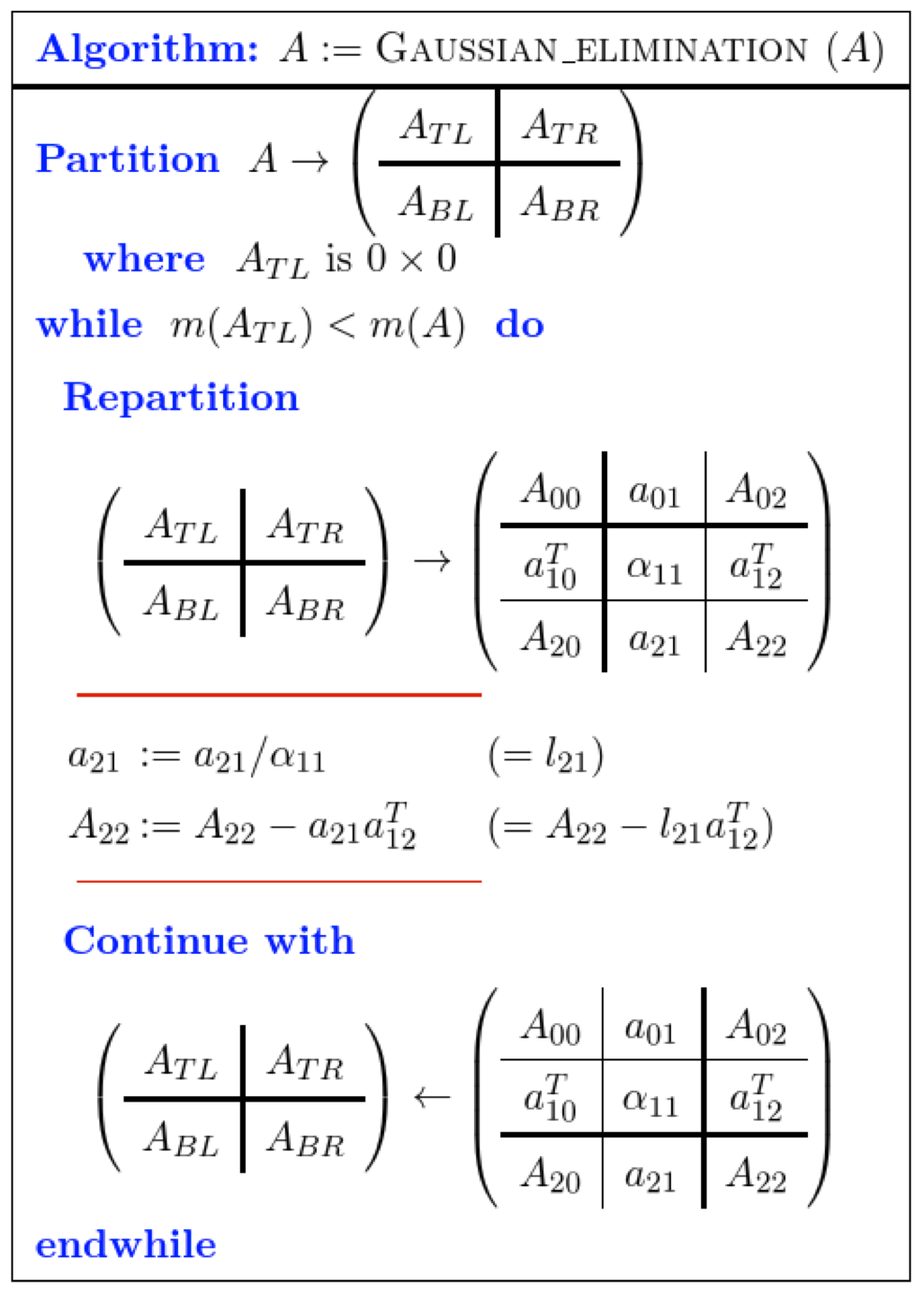
Now, let's implement the Gaussian Elimination routine from 6.2.5
Here is the algorithm:
Important: if you make a mistake, rerun ALL cells above the cell in which you were working before you rerun the one in which you are working.
Create the routine
GaussianElimination( A )
with the Spark webpage for the algorithm given above.
Recall from the explanation that a Gauss transform needs to be computed so that
$ \left( \begin{array}{c | c } 1 & 0 \\ \hline -l_{21} & I \end{array} \right) \left( \begin{array}{c | c } \alpha_{11} & a_{12}^T \\ \hline a_{21} & A_{22} \end{array} \right) = \left( \begin{array}{c | c } \alpha_{11} & a_{12}^T \\ \hline 0 & A_{22} - l_{21} a_{12}^T \end{array} \right) $. Notice that it must be true that $ l_{21} := a_{21} / \alpha_{11} $ in order to get a zero in the bottom left quadrant of the resulting matrix.
It follows from partitioned matrix multiplication that we must update $ A_{22} := A_{22} - l_{21} * a_{12}^T $.
# Insert routine here
Test the routine
Important: if you make a mistake, rerun ALL cells above the cell in which you were working before you rerun the one in which you are working.
# recreate matrix A
A = L * U

# recreate the right-hand side
b = A * xold

# apply Gaussian elimination to matrix A
GaussianElimination_unb( A )
Compare the overwritten matrix, $ A $, to the original matrices, $ L $ and $ U $. The upper triangular part of $ A $ should equal $ U $ and the strictly lower triangular part of $ A $ should equal the strictly lower triangular part of $ L $. The reason for this will become clear in Unit 6.3.1.
Important: if you make a mistake, rerun ALL cells above the cell in which you were working before you rerun the one in which you are working.
print( A )
print( 'Original L' )
print( L )
print( 'Original U' )
print( U )
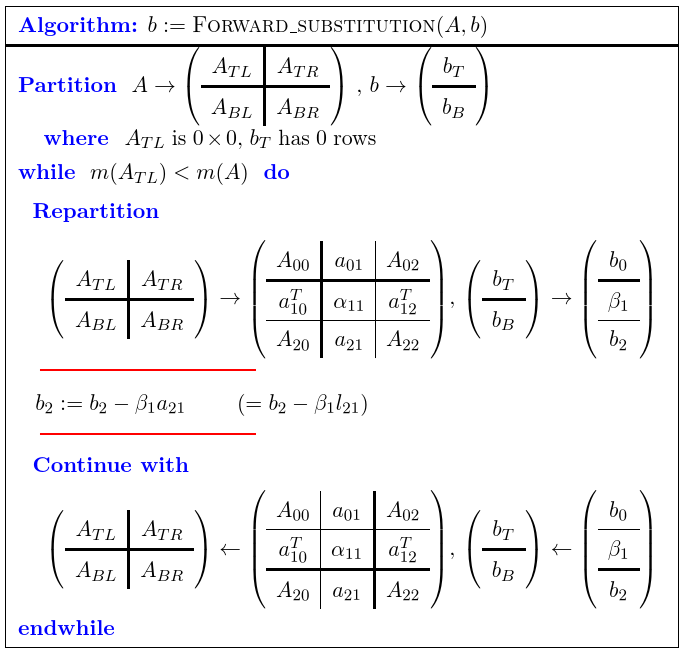
Now, let's implement the forward substitution routine from 6.2.5
Here is the algorithm:
Important: if you make a mistake, rerun ALL cells above the cell in which you were working before you rerun the one in which you are working.
Create the routine
ForwardSubstitution_unb( A, b )
with the Spark webpage for the algorithm.
# Insert code here
Apply the Gauss transforms to the right-hand side
Important: if you make a mistake, rerun ALL cells above the cell in which you were working before you rerun the one in which you are working.
print( A )
print( b )
ForwardSubstitution_unb( A, b )

print( 'updated b' )
print( b )
Now, perform back substitution
Important: if you make a mistake, rerun ALL cells above the cell in which you were working before you rerun the one in which you are working.
x[ 3 ] = b[ 3 ] / A[ 3,3 ]
x[ 2 ] = ( b[ 2 ] - A[ 2,3 ] * x[ 3 ] ) / A[ 2,2 ]
x[ 1 ] = ( b[ 1 ] - A[ 1,2 ] * x[ 2 ] - A[ 1,3 ] * x[ 3 ] ) / A[ 1,1 ]
x[ 0 ] = ( b[ 0 ] - A[ 0,1 ] * x[ 1 ] - A[ 0,2 ] * x[ 2 ]- A[ 0,3 ] * x[ 3 ] ) / A[ 0,0 ]
print( 'x = ' )
print( x )

print( 'x - xold' )
print( x - xold )
x - xold should yield a zero vector