This notebook will cover the assumed knowledge of pandas. Here's a few questions to check if you already know the material in this notebook.
- Does a NumPy array have a single dtype or multiple dtypes?
- Why is broadcasting useful?
- How do you slice a DataFrame by row label?
- How do you select a column of a DataFrame?
- Is the Index a column in the DataFrame?
If you feel pretty comfortable with those, go ahead and skip this notebook. Answers are at the end. We'll meet up at the next notebook.
Aside: IPython Notebook
- two modes command and edit
- command -> edit:
Enter - edit -> command:
Esc
- command -> edit:
h: Keyboard Shortcuts: (from command mode)j/k: navigate cellsshift+Enterexecutes a cell
Outline:
Numpy Foundation
pandas is built atop NumPy, historically and in the actual library. It's helpful to have a good understanding of some NumPyisms. Speak the vernacular.
ndarray
The core of numpy is the ndarray, N-dimensional array. These are homogenously-typed, fixed-length data containers.
NumPy also provides many convenient and fast methods implemented on the ndarray.
from __future__ import print_function

import numpy as np
import pandas as pd

x = np.array([1, 2, 3])
x
array([1, 2, 3])
x.dtype
dtype('int64')
y = np.array([[True, False], [False, True]])
y
array([[ True, False],
       [False,  True]], dtype=bool)
y.shape
(2, 2)
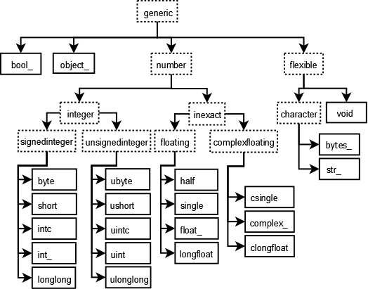
dtypes
Unlike python lists, NumPy arrays care about the type of data stored within. The full list of NumPy dtypes can be found in the NumPy documentation.
We sacrifice the convinience of mixing bools and ints and floats within an array for much better performance.
However, an unexpected dtype change will probably bite you at some point in the future.
The two biggest things to remember are
- Missing values (NaN) cast integer or boolean arrays to floats
- the object dtype is the fallback
You'll want to avoid object dtypes. It's typically slow.
Broadcasting
It's super cool and super useful. The one-line explanation is that when doing elementwise operations, things expand to the "correct" shape.
# add a scalar to a 1-d array
x = np.arange(5)
print('x:  ', x)
print('x+1:', x + 1, end='\n\n')

y = np.random.uniform(size=(2, 5))
print('y:  ', y,  sep='\n')
print('y+1:', y + 1, sep='\n')
x:   [0 1 2 3 4]
x+1: [1 2 3 4 5]

y:
[[ 0.27612315  0.18577684  0.9610967   0.92516769  0.43423458]
 [ 0.41534299  0.58181509  0.49158344  0.43734366  0.09782122]]
y+1:
[[ 1.27612315  1.18577684  1.9610967   1.92516769  1.43423458]
 [ 1.41534299  1.58181509  1.49158344  1.43734366  1.09782122]]
Since x is shaped (5,) and y is shaped (2,5) we can do operations between them.
x * y
array([[ 0.        ,  0.18577684,  1.9221934 ,  2.77550307,  1.73693832],
       [ 0.        ,  0.58181509,  0.98316688,  1.31203099,  0.3912849 ]])
Without broadcasting we'd have to manually reshape our arrays, which quickly gets annoying.
x.reshape(1, 5).repeat(2, axis=0) * y
array([[ 0.        ,  0.18577684,  1.9221934 ,  2.77550307,  1.73693832],
       [ 0.        ,  0.58181509,  0.98316688,  1.31203099,  0.3912849 ]])
Pandas
We'll breeze through the basics here, and get onto some interesting applications in a bit. I want to provide the barest of intuition so things stick down the road.
Why pandas
NumPy is great. But it lacks a few things that are conducive to doing statisitcal analysis. By building on top of NumPy, pandas provides
- labeled arrays
- heterogenous data types within a table
- better missing data handling
- convenient methods
- more data types (Categorical, Datetime)
Data Structures
This is the typical starting point for any intro to pandas. We'll follow suit.
The DataFrame
Here we have the workhorse data structure for pandas. It's an in-memory table holding your data, and provides a few conviniences over lists of lists or NumPy arrays.
import numpy as np
import pandas as pd
# Many ways to construct a DataFrame
# We pass a dict of {column name: column values}
np.random.seed(42)
df = pd.DataFrame({'A': [1, 2, 3], 'B': [True, True, False],
                   'C': np.random.randn(3)},
                  index=['a', 'b', 'c'])  # also this weird index thing
df
| A | B | C | |
|---|---|---|---|
| a | 1 | True | 0.496714 |
| b | 2 | True | -0.138264 |
| c | 3 | False | 0.647689 |
from IPython.display import Image

Image('dataframe.png')

Selecting
Our first improvement over numpy arrays is labeled indexing. We can select subsets by column, row, or both. Column selection uses the regular python __getitem__ machinery. Pass in a single column label 'A' or a list of labels ['A', 'C'] to select subsets of the original DataFrame.
# Single column, reduces to a Series
df['A']
a    1
b    2
c    3
Name: A, dtype: int64
cols = ['A', 'C']
df[cols]
| A | C | |
|---|---|---|
| a | 1 | 0.496714 |
| b | 2 | -0.138264 |
| c | 3 | 0.647689 |
For row-wise selection, use the special .loc accessor.
df.loc[['a', 'b']]
| A | B | C | |
|---|---|---|---|
| a | 1 | True | 0.496714 |
| b | 2 | True | -0.138264 |
When your index labels are ordered, you can use ranges to select rows or columns.
df.loc['a':'b']
| A | B | C | |
|---|---|---|---|
| a | 1 | True | 0.496714 |
| b | 2 | True | -0.138264 |
Notice that the slice is inclusive on both sides, unlike your typical slicing of a list. Sometimes, you'd rather slice by position instead of label. .iloc has you covered:
df.iloc[0:2]
| A | B | C | |
|---|---|---|---|
| a | 1 | True | 0.496714 |
| b | 2 | True | -0.138264 |
This follows the usual python slicing rules: closed on the left, open on the right.
As I mentioned, you can slice both rows and columns. Use .loc for label or .iloc for position indexing.
df.loc['a', 'B']
True
Pandas, like NumPy, will reduce dimensions when possible. Select a single column and you get back Series (see below). Select a single row and single column, you get a scalar.
You can get pretty fancy:
df.loc['a':'b', ['A', 'C']]
| A | C | |
|---|---|---|
| a | 1 | 0.496714 |
| b | 2 | -0.138264 |
Summary
- Use
[]for selecting columns - Use
.loc[row_lables, column_labels]for label-based indexing - Use
.iloc[row_positions, column_positions]for positional index
I've left out boolean and hierarchical indexing, which we'll see later.
Series
You've already seen some Series up above. It's the 1-dimensional analog of the DataFrame. Each column in a DataFrame is in some sense a Series. You can select a Series from a DataFrame in a few ways:
# __getitem__ like before
df['A']
a    1
b    2
c    3
Name: A, dtype: int64
# .loc, like before
df.loc[:, 'A']
a    1
b    2
c    3
Name: A, dtype: int64
# using `.` attribute lookup
df.A
a    1
b    2
c    3
Name: A, dtype: int64
You'll have to be careful with the last one. It won't work if you're column name isn't a valid python identifier (say it has a space) or if it conflicts with one of the (many) methods on DataFrame. The . accessor is extremely convient for interactive use though.
You should never assign a column with . e.g. don't do
# bad
df.A = [1, 2, 3]
It's unclear whether your attaching the list [1, 2, 3] as an attirbute of df, or whether you want it as a column. It's better to just say
df['A'] = [1, 2, 3]
# or
df.loc[:, 'A'] = [1, 2, 3]
Series share many of the same methods as DataFrames.
Index
Indexes are something of a peculiarity to pandas.
First off, they are not the kind of indexes you'll find in SQL, which are used to help the engine speed up certain queries.
In pandas, Indexes are about lables. This helps with selection (like we did above) and automatic alignment when performing operations between two DataFrames or Series.
R does have row labels, but they're nowhere near as powerful (or complicated) as in pandas. You can access the index of a DataFrame or Series with the .index attribute.
df.index
Index(['a', 'b', 'c'], dtype='object')
There are special kinds of Indexes that you'll come across. Some of these are
MultiIndexfor multidimensional (Hierarchical) labelsDatetimeIndexfor datetimesFloat64Indexfor floatsCategoricalIndexfor, you guessed it,Categoricals
We'll talk a lot more about indexes. They're a complex topic and can introduce headaches.
@gjreda @treycausey in some cases row indexes are the best thing since sliced bread, in others they simply get in the way. Hard problem
— Wes McKinney (@wesmckinn) December 22, 2014Pandas, for better or for worse, does usually provide ways around row indexes being obstacles. The problem is knowing when they are just getting in the way, which mostly comes by experience. Sorry.
Answers
- Does a NumPy array have a single dtype or multiple dtypes?
- NumPy arrays are homogenous: they only have a single dtype (unlike DataFrames).
You can have an array that holds mixed types, e.g. np.array(['a', 1]), but the
dtype of that array is object, which you probably want to avoid.
2. Why is broadcasting useful?
- It lets you perform operations between arrays that are compatable, but not nescessarily identical,
in shape. This makes your code cleaner. 3. How do you slice a DataFrame by row label?
- Use
.loc[label]. For position based use.iloc[integer].
- How do you select a column of a DataFrame?
- Standard
__getitem__:df[column_name]
- Is the Index a column in the DataFrame?
- No. It isn't included in any operations (
mean, etc). It can be inserted as a regular
column with df.reset_index().