Clustering and Latent Variable Models, MLSS 2015
Authors: Daniel Steinberg & Brian Thorne
Institute: NICTA
Clustering
Regression and classification are very useful for when we have some targets/labels for training, however, what about situations where we do not have targets/labels? This is where unsupervised methods such as dimensionality reduction and clustering can help us out by trying to infer categories from the data (clustering) or a low dimensional representation of the data (dimensionality reduction). We have already seen a simple dimensionality reduction technique, PCA, in the first tutorial. In this tutorial we will look at some clustering algorithms and a latent variable model that can be both interpreted as clustering and dimensionality reduction
Clustering is one of the oldest data exploration methods. The objective is for an algorithm to discover sets of similar points, or observations, within a larger dataset. These sets are called clusters. Similarity is almost always characterised by some distance function between observations, such as Euclidean $\ell_2$. Some of the more simple algorithms require the number of clusters to be specified in advance, while others can also infer this from the data, usually given other assumptions. K-means was one of the first and still most popular algorithms designed for this task.
K-means
The objective of K-means clustering is to find $K$ clusters of observations within a dataset of $N$ observations, $\obsall = \cbrac{\obsind_n}^N_{n=1}$, where $\obsind_n \in \real{D}$. These clusters are characterised by their means, $\mathbf{M} = \cbrac{\gausmean_k}^K_{k=1}$ where $\gausmean_k \in \real{D}$. Each observation is assigned to a cluster mean using an integer label $\olabind_n \in \cbrac{1,\ldots,K}$, and $\olaball = \cbrac{\olabind_n}^N_{n=1}$. The objective of K-means is to minimise the square loss, or reconstruction error, \begin{equation} \min_{\mathbf{M},\olaball} \sum^N_{n=1} \sum^K_{k=1} \indic{\olabind_n = k} \norm{\obsind_n - \gausmean_k}{2}^2. \end{equation} Here $\indic{\cdot}$ is an indicator function that evaluates to 1 when the condition in the brackets is true, and 0 otherwise. $\norm{\cdot}{2}$ is an $\ell_2$ norm, or Euclidean distance. This is solved with two simple alternating steps. The first is the assignment step; \begin{equation} \olabind_n = \argmin{k} \norm{\obsind_n - \gausmean_k}{2}^2, \end{equation} the next is the update step; \begin{equation} \gausmean_k = \frac{\sum_n \indic{\olabind_n = k} \obsind_n} {\sum_n \indic{\olabind_n = k}}. \end{equation} These two steps are iterated until the square loss in objective has converged, and that's it! This is sometimes also referred to as the Expectation-Maximisation (EM) algorithm because of its relationship to Gausian mixture models - more on this soon.
Unfortunately this is not guaranteed to converge to a global minimum of the objective function, and usually many random initialisations (random choices of $\obsind_n$ for the initial $\gausmean_k$) have to be attempted to find the best solution. This algorithm is very fast in practice though. Another disadvantage is that the number of clusters, $K$, has to be specified in advance. Perhaps more of a concern is that clusters are assumed to be essentially spherical in shape because of the Euclidean distance used, which is quite often an over-simplification. It is also useful to have probabilistic assignments, $\probC{\olabind_n = k}{\obsind_n}$ rather than hard assignments. Gaussian mixture models solve these last two problems.
Exercises
1) Have a go at calculating the hard assignments, $\olabind_n$, for the data, $\obsind_n$, from the initial means/centres, $\gausmean_k$, provided. Also try to plot the results using the provided function.
# Importing some libraries and modules
%pylab inline

import numpy as np
import matplotlib.pyplot as plt
import tututils as tut
Populating the interactive namespace from numpy and matplotlib
WARNING: pylab import has clobbered these variables: ['dist']
`%matplotlib` prevents importing * from pylab and numpy
# Load X from a dataset generation function from tututils
X = tut.load_2d_simple()
K = 3  # There are three clusters in this dataset
N = X.shape[0]
k_means_cluster_centers = X[np.random.randint(0, N, size=K), :]

# Now calculate Z from X and k_means_cluster_centers.
# Tip: consider using numpy's argmin()

#### SOLUTION CODE (TEST)
dist = np.zeros((X.shape[0], K))
for k in range(K):
    dist[:, k] = ((X - k_means_cluster_centers[k])**2).sum(axis=1)
k_means_labels = dist.argmin(axis=1)
#### END SOLUTION CODE (TEST)

# Check your answer by plotting the clusters:
tut.plot_2d_clusters(X, k_means_labels, k_means_cluster_centers)

2) Now have a go at calculating the cluster means, $\gausmean_k$, given the cluster assignments, $\olabind_n$, calculated previously. Again, plot the results using the provided function.
# Calculate k_means_cluster_centers from X and k_means_labels

#### SOLUTION CODE (TEST)
k_means_cluster_centers = [X[k_means_labels == k, :].mean(axis=0) for k in range(K)]
#### END SOLUTION CODE (TEST)

# Check your answer by plotting the clusters:
# TIP: You may need to re-do the labels to make the vornoi cells match the labels

#### SOLUTION CODE (TEST)
dist = np.zeros((X.shape[0], K))
for k in range(K):
    dist[:, k] = ((X - k_means_cluster_centers[k])**2).sum(axis=1)
k_means_labels = dist.argmin(axis=1)
#### END SOLUTION CODE (TEST)

tut.plot_2d_clusters(X, k_means_labels, k_means_cluster_centers)

3) Let's tie it all together now, and implement the K-means clustering algorithm in its entirety, you can use the following code as a template, or you can make your own from scratch. Once the algorithm works and converges, plot the final result to see how it differs from the above plots.
# Funcion template -- fill in the gaps
def kmeans(X, K, maxit=100):

    # initialise
    N, D = X.shape
    M = X[np.random.randint(0, N, size=K), :]
    obj = np.finfo(float).max

    #### SOLUTION CODE (TEST)
    dist = np.zeros((N, K))
    #### END SOLUTION CODE (TEST)

    for i in range(maxit):
        objo = obj

        # TODO: E-step, update indicators
        # TODO: M-step, update means
        # TODO: Calculate loss function i.e. obj =

        #### SOLUTION CODE (TEST)
        for k in range(K):
            dist[:, k] = ((X - M[k, :])**2).sum(axis=1)
        Z = dist.argmin(axis=1)

        M = np.array([X[Z == k, :].mean(axis=0) for k in range(K)])

        obj = ((X - M[Z, :])**2).sum()
        #### END SOLUTION CODE (TEST)

        if (objo - obj) / objo < 1e-5:
            break

    return Z, M
# Call your kmeans function on the data

#### SOLUTION CODE (TEST)
k_means_labels, k_means_cluster_centers = kmeans(X, 3)
#### END SOLUTION CODE (TEST)

# plot the final result
tut.plot_2d_clusters(X, k_means_labels, k_means_cluster_centers)

4) K-means is often used to quantise various datasets, for instance, we can use it to "compress" images by clustering the RGB data into fewer colors. Open up the kmeans-image notebook to run this example (if you are running out of time, feel free to move on).
Gaussian Mixture Models
Gaussian mixture models (GMMs) can be viewed as a probabilistic generalisation of K-means (i.e. probabilistic cluster assignments) with the added ability to learn ellipsoidal clusters. In a GMM each observation is distributed according to a weighted sum of $K$ multivariate Gaussian distributions; \begin{equation} \obsind_n \sim \sum^K_{k=1} \wgtmix_k \gausC{\obsind_n}{\gausmean_k, \gauscov_k}. \end{equation} Here $\wgtind = [\wgtmix_1,\ldots,\wgtmix_k,\ldots,\wgtmix_K]\transpose$ and $\wgtmix_k \in [0,1]$, with $\sum_k \wgtmix_k = 1$. $\gauscov_k$ is a covariance matrix that describes the "spread" of uncertainty in the Gaussian distribution, which is usually ellipsoidal in shape. Here is an example of what a GMM may look like in two dimensions (we have plotted the 65% probability mass contours for the Gaussians):
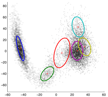
The weights of each Gaussian have in this mixture have not been explicitly represented, but they are implicit in the amount of observations (darkness of the voxels) they are modelling.
The following is a brief explanation of a GMM, it is more complex than K-means, so do not worry if you don't understand it fully - a full grasp of GMMs is not required for the exercises.
We need a way to explicitly assign observations to mixtures or clusters. The same latent variable, $\olabind_n$, used in K-means is introduced here as an auxiliary variable for this purpose, by inducing the following conditional relationship; \begin{equation} \probC{\obsind_n}{\olabind_n} = \prod^K_{k=1} \gausC{\obsind_n}{\gausmean_k, \gauscov_k}^\indic{\olabind_n=k}, \end{equation} so given a cluster, $\probC{\obsind_n}{\olabind_k=k} = \gausC{\obsind_n} {\gausmean_k, \gauscov_k}$. Now it can be seen that each cluster is modelled as a single Gaussian with a full covariance matrix. This auxiliary variable is itself distributed according to a Categorical distribution (same as a Multinomial distribution but with only one observation); \begin{equation} \olabind_n \sim \categ{\wgtind} = \prod^K_{k=1} \wgtmix_k^\indic{\olabind_n = k}. \end{equation} The joint distribution for this GMM can be written as, \begin{equation} \prob{\obsall, \olaball} = \prod^N_{n=1} \categC{\olabind_n}{\wgtind} \prod^K_{k=1} \gausC{\obsind_n}{\gausmean_k, \gauscov_k}^\indic{\olabind_n=k}. \end{equation}
Now we need an algorithm that can learn the labels, $\olabind_n$, cluster parameters, $\gausmean_k$ and $\gauscov_k$, and mixture weights, $\wgtind$. Such an algorithm can be derived by maximising the log-likelihood of the data, \begin{equation} \log \prob{\obsall} = \sum_{n=1}^N \log \sum^K_{k=1} \wgtmix_k \gausC{\obsind_n}{\gausmean_k, \gauscov_k}, \end{equation} which is acheived by setting the partial derivative of this equation with respect to each parameter and the labels in turn to zero and solving for the parameters/labels.
Firstly, maximising the log-likelihood with respect to $\olabind_n$, yields; \begin{equation} \probC{\olabind_n = k}{\obsind_n} = \frac{\wgtmix_k \gausC{\obsind_n}{\gausmean_k, \gauscov_k}} {\sum_l \wgtmix_l \gausC{\obsind_n}{\gausmean_l, \gauscov_l}}, \end{equation} This is known as the expectation step, since the labels are probabilistically assigned their expected value given the observations and cluster parameters.
Next, the parameters can be found by maximising the log-likelihood with respect to each parameter; \begin{align} \gausmean_k &= \frac{\sum_n \probC{\olabind_n=k}{\obsind_n} \obsind_n} {\sum_n \probC{\olabind_n=k}{\obsind_n}}, \\ \gauscov_k &= \frac{1}{\sum_n \probC{\olabind_n=k}{\obsind_n}} \sum^N_{n=1} \probC{\olabind_n = k}{\obsind_n} (\obsind_n - \gausmean_k)(\obsind_n - \gausmean_k)\transpose, \\ \wgtmix_k &= \sum^N_{n=1} \frac{\probC{\olabind_n = k}{\obsind_n}} {\sum_k \probC{\olabind_n = k}{\obsind_n}}. \end{align} This is called the maximisation step, because the value of the log-likelihood is maximised with respect to the parameters given the estimated latent variables. These two steps are iterated until the log-likelihood converges. This is known as the expectation-maximisation EM algorithm. For all intents and purposes it is the same algorithm used to learn K-means.
Unfortunately this algorithm has a few drawbacks. Like K-means, it is only guaranteed to converge to a local maximum of the likelihood function. Also, the Gaussian cluster updates require a full $D \times D$ covariance matrix inversion, which has an $\bigO{D^3}$ computational cost. This can be circumvented by using diagonal covariance Gaussian clusters, or other distributions such as Multinomial, that have only $\bigO{D}$ computational cost. Though some expressive power is lost since inter-dimensional correlation is not modelled.
Another drawback is that this algorithm still cannot choose $K$. One way to allow the EM algorithm to choose $K$ is to include a penalty, or regulariser, for having too many parameters. In this way the maximum-likelihood fitting objective can be traded off against a model complexity penalty. Some popular penalties are the Akaike information criterion and the Bayesian information criterion. These criterion tend to under-penalise model complexity, and are sometimes computationally costly to calculate. Another way to choose $K$ is to use a fully Bayesian treatment, where we place prior distributions on the parameters (e.g. mean, covariance and weights), and then optimise the log marginal likelihood of the model, which also naturally incorporates a penalty for complexity. In the case of mixture models, the Bayesian learning algorithms can have very little additional computational cost compared to EM. For more information on EM algorithms for mixture models, see (Bishop, 2006) Chapters 9 and 10.
Exercises
5) Run K-means on the following dataset with 3 clusters and visualise the results
# Load X from a dataset generation function from tututils
X, truth = tut.load_2d_hard()

#### SOLUTION CODE (TEST)
labels, centres = kmeans(X, 3)
#### END SOLUTION CODE (TEST)

tut.plot_2d_clusters(X, labels, centres)

6) Now cluster the same data with a GMM, why do you think these results are so different?
from sklearn.mixture import GMM

# Hint, use covariance_type='full' option

#### SOLUTION CODE (TEST)
gmm = GMM(n_components=3, covariance_type='full')
gmm.fit(X)
labels = gmm.predict(X)
means = gmm.means_
covs = gmm.covars_
#### END SOLUTION CODE (TEST)

# Plot
tut.plot_2d_GMMs(X, labels, means, covs)

7) Ok, now try K-means and GMMs with 6 clusters and plot the results, what happens?
# Kmeans clustering

#### SOLUTION CODE (TEST)
labels_k, centres = kmeans(X, 6)
#### END SOLUTION CODE (TEST)

tut.plot_2d_clusters(X, labels_k, centres)

# GMM clustering

#### SOLUTION CODE (TEST)
gmm = GMM(n_components=6, covariance_type='full')
gmm.fit(X)
labels_g = gmm.predict(X)
means = gmm.means_
covs = gmm.covars_
#### END SOLUTION CODE (TEST)

# Plot
tut.plot_2d_GMMs(X, labels_g, means, covs)


As you can see, if we don't have a reasonable idea of the number of clusters before we begin, we may not get great results. As mentioned before, there are clustering methods that can also infer the number of clusters, some of which include:
- variational Bayes Gaussian mixture models (VBGMM) (Attias, 1999; Bishop, 2006)
- Dirichlet process or infinite Gaussian mixture models (Rasmussen, 1999)
- Spectral clustering (von Luxburg, 2007)
- DBSCAN
The scikit learn clustering documentation also has a nice summary of the capabilites of many popular clustering algorithms, including a demonstration of the types of cluster shapes that can be modelled:

8) If we have some kind of ground truth labels (as we do in the truth variable from ex. 5) we can get a measure of a clustering solutions validity from various measures. One of the more popular and robust measure is Normalised Mutual Information (NMI). What is nice about this measure is that the number of cluster labels do not have to match the number of ground truth labels unlike many classification metrics.
Run both K-means and the GMM for varying number of clusters (1 to 6), and plot their NMI vs. number of clusters.
from sklearn.metrics import normalized_mutual_info_score

Ks = range(1, 7)
NMI_k = []
NMI_g = []

for k in Ks:

    # Kmeans clustering

    #### SOLUTION CODE (TEST)
    labels_k, _ = kmeans(X, k)
    NMI_k.append(normalized_mutual_info_score(truth, labels_k))
    #### END SOLUTION CODE (TEST)

    #NMI_k.append(TODO)

    # GMM clustering

    #### SOLUTION CODE (TEST)
    gmm = GMM(n_components=k, covariance_type='full')
    gmm.fit(X)
    labels_g = gmm.predict(X)
    NMI_g.append(normalized_mutual_info_score(truth, labels_g))
    #### END SOLUTION CODE (TEST)

    #NMI_g.append(TODO)

#### SOLUTION CODE (TEST)
plt.plot(Ks, NMI_k, 'r*-')
plt.plot(Ks, NMI_g, 'bo-')
plt.legend(['K-means', 'GMM'], loc='lower right')
plt.xlabel('k')
plt.ylabel('NMI')
plt.grid(True)
#### END SOLUTION CODE (TEST)

In reality, if we had all, or even some, of the labels like this it would more prudent to use a supervised classification method and the corresponding supervised classification performance metrics (like percent classification error, F-measure, etc). However clustering is still useful as a data exploration strategy, as well as a feature creation method for classification -- it is quite common to see kmeans with (very) large K being used to cluster inputs to a linear classifier to improve classification performance, among other strategies.
As a final note, I would recommend against using the implementation of Variational Bayes GMMs and Dirichlet Process GMMs in scikit learn for now, I have never had much luck with them, and could not even get them to fit the above datasets. If you would like to test out these algorithms, I have a much more robust implementation in libcluster.
Topic Models
The purpose of topic modelling is to generally learn some low-dimensional representation of a large collection of textual documents, called a corpus. The representation can be used to summarize a corpus, or for retrieval of documents that are similar to a query document.
Typically topic models are learned by analysing the distribution of words within a corpus, in particular how they cluster together within documents that have similar subjects. These clusters of words are referred to as "topics", and documents may comprise several topics in different amounts. These topics are essentially the low-dimensional representation of documents learned by topic models.
Latent Dirichlet Allocation
One of the most well known topic models is latent Dirichlet allocation (LDA) (Blei, 2003), also known as multinomial PCA (Buntine, 2002).
Typically a corpus is broken down as follows:
- There are $J$ documents in a corpus,
- there are $N_j$ words in each document, $j$,
- a word, $\sobsind_{nj}$, is represented as an index into a vocabulary, i.e. $\sobsind_{jn} \in \cbrac{1,\ldots,D}$ where $D$ is the size of the vocabulary.
So we can think of our whole dataset (corpus) being made up of sub-datasets (documents), $\obsall = \cbrac{\obsall_j}^J_{j=1}$, which are collections of words in each document, $\obsall_j = \cbrac{\sobsind_{jn}}^{N_j}_{n=1}$. This is called a bag of words model, because order of the words is assumed unimportant. This simplifying assumption is known as the exchangeability assumption.
LDA goes on to model a corpus as follows:
- Each document, $j$, is represented as a low-dimensional proportion of $K$ topics $$\wgtind_j \sim \dir{\dirall},$$ where $\wgtind_j = \cbrac{\wgtmix_{j1}, \ldots, \wgtmix_{jK}}$ and $\sum_k \wgtmix_k = 1$.
- Each word, $\sobsind_{jn}$, is drawn from a per-topic vocabulary, represented as a categorical distribution, in proportion to the per-document topic mixture $$\sobsind_{jn} \sim \sum^K_{k=1} \wgtmix_{jk} \categC{\sobsind_{jn}}{\mwgtind_k},$$ where $\mwgtind_k$ are the parameters of the topic categorical distribution (which are also vector of weights that sum to one).
This is very similar to the GMM we saw before, the differences being that we now have Categorical clusters as opposed to Gaussian clusters, and that we have mixture weights, $\wgtmix_{jk}$, specific to each document. What is nice is that the clusters/topics are shared over all documents. This enables us to view these topic/cluster weights, $\wgtind_j$ as a low-dimensional description of the original document, i.e. a mixture of topics!
This is a Bayesian model and sometimes has a prior also placed on $\mwgtind_k \sim \dir{\dircall}$, which is called smoothed LDA.
LDA can use fast sampling techniques, such as Gibbs sampling, or approximate marginal likelihood techniques, such as variational Bayes, for learning the model latent variables and hyper-parameters. Limitations have also been found with LDA. For example, it is not effective in choosing the number of topics ($K$), and the symmetric Dirichlet prior over topic weights, has been found to be too restrictive. Hierarchical Dirichlet processes (Teh, 2006) have been developed to overcome both of these issues (but is beyond the scope of this tutorial).
9) For this exercise we will run LDA on a fairly standard dataset comprising news articles from Reuters.
For this exercise you'll need this python LDA package. It can be installed via pip easily:
$ sudo pip install lda # you may need to use your distribution's version of pip (pip3, pip-python3, conda etc)
Also, this may require you to also manually install the pbr python package (also through pip).
Now, essentially follow the getting started tutorial in the documentation. It is worth noting that this dataset has undergone quite a bit of pre-processing, such as removing certain "stop" words so the resultant topics are not inundated with common and uninformative words likes "and".
import lda
import lda.datasets

# Load the data
X = lda.datasets.load_reuters()
vocab = lda.datasets.load_reuters_vocab()

# TODO: create the LDA object with 20 topics
#model =

#### SOLUTION CODE (TEST)
model = lda.LDA(n_topics=20, n_iter=500, random_state=1)
#### END SOLUTION CODE (TEST)

# TODO: fit the LDA object to data

#### SOLUTION CODE (TEST)
model.fit(X)
#### END SOLUTION CODE (TEST)

# Print out a selection of topics
topic_word = model.topic_word_  # model.components_ also works
n_top_words = 8
for i, topic_dist in enumerate(topic_word):
    topic_words = np.array(vocab)[np.argsort(topic_dist)][:-n_top_words:-1]
    print('Topic {}: {}'.format(i, ' '.join(topic_words)))
Topic 0: church people told years last year time
Topic 1: elvis music fans york show concert king
Topic 2: pope trip mass vatican poland health john
Topic 3: film french against france festival magazine quebec
Topic 4: king michael romania president first service romanian
Topic 5: police family versace miami cunanan west home
Topic 6: germany german war political government minister nazi
Topic 7: harriman u.s clinton churchill ambassador paris british
Topic 8: yeltsin russian russia president kremlin moscow operation
Topic 9: prince queen bowles church king royal public
Topic 10: simpson million years south irish churches says
Topic 11: charles diana parker camilla marriage family royal
Topic 12: east peace prize president award catholic timor
Topic 13: order nuns india successor election roman sister
Topic 14: pope vatican hospital surgery rome roman doctors
Topic 15: mother teresa heart calcutta missionaries hospital charity
Topic 16: bernardin cardinal cancer church life catholic chicago
Topic 17: died funeral church city death buddhist israel
Topic 18: museum kennedy cultural city culture greek byzantine
Topic 19: art exhibition century city tour works madonna
10) Try setting the number of topics found to different numbers, and see what impact there is on the results.
# TODO, repeat above, but with a different number of topics
Bibliography
(Bishop, 2006) C. M. Bishop. Pattern Recognition and Machine Learning. Springer Science+Business Media, Cambridge, UK, 2006.
(Blei, 2003) D. M. Blei and M. I. Jordan. Modeling annotated data. In Proceedings of the 26th annual international ACM SIGIR conference on Research and development in informaion retrieval, SIGIR ’03, pages 127–134, New York, NY, USA, 2003. ACM. ISBN 1-58113-646-3.
(Buntine, 2002) W. Buntine. Variational extensions to EM and multinomial PCA. Machine Learning: ECML 2002, pages 23–34, 2002.
(Teh, 2006) Y. W. Teh, M. I. Jordan, M. J. Beal, and D. M. Blei. Hierarchical Dirichlet processes. Journal of the American Statistical Association, 101(476):1566–1581, 2006.