SLIP Model Example
MCHE 513: Intermediate Dynamics
Dr. Joshua Vaughan
joshua.vaughan@louisiana.edu
http://www.ucs.louisiana.edu/~jev9637/
The Spring Loaded Inverted Pendulum (SLIP) model, shown in Figure 1, is often used to model walking, running, or jumping of animals, including humans. The system consists of a point mass, $m$, connected to a spring of stiffness $k$. The rotation of the inverted pendulum is represented by $\theta$ and the length of the spring by $R$. The equilibrium length of the spring is $L_0$.
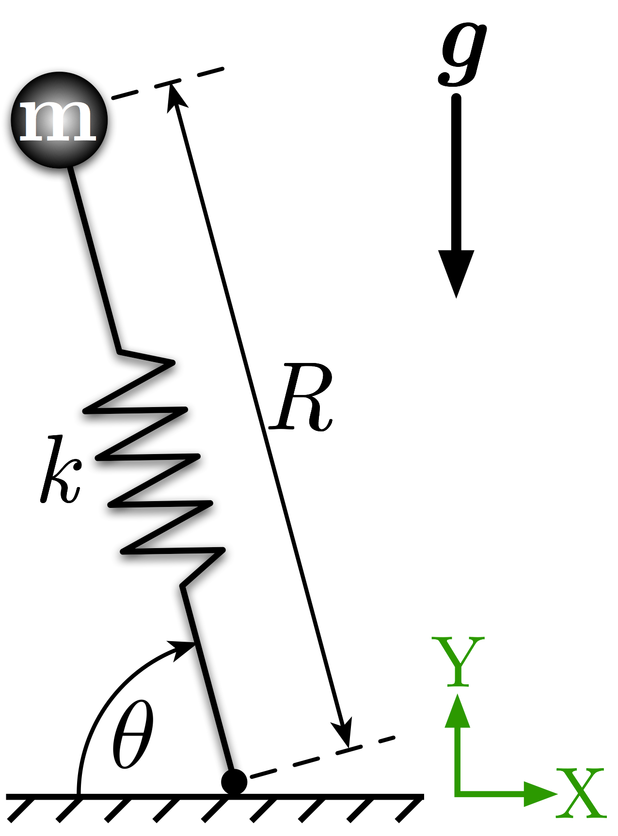
Figure 1: Spring Loaded Inverted Pendulum (SLIP) Model
The spring is often modeled as free to leave the ground, in order to represnt the "flight" phase of walking or running (i.e. When the leg is in the air.). Here, we'll just model the "stance" portion, when the spring is in contact with the gorund.
# Import the SymPy Module
import sympy

# Import the necessary sub-modules and methods for dynamics
from sympy.physics.mechanics import dynamicsymbols
from sympy.physics.mechanics import LagrangesMethod, Lagrangian
from sympy.physics.mechanics import Particle, Point, ReferenceFrame

# initiate better printing of SymPy results
sympy.init_printing()
# Define the genearlized coordinate
R, theta = dynamicsymbols('R theta')

# Also define the first derivative
R_dot, theta_dot = dynamicsymbols('R theta', 1)

# Define the symbols for the other paramters
m, g, k, l0, t = sympy.symbols('m g k L_0 t')
# Define the Newtonian reference frame
N = ReferenceFrame('N')

# Define a body-fixed frame along the pendulum, with y aligned from m to the pin
A = N.orientnew('A', 'Axis', [-(sympy.pi/2 - theta), N.z])

# Define the points and set its velocity
P = Point('P')
P.set_vel(N, R * theta_dot * A.x + R_dot * A.y)

mp = Particle('mp', P, m)

mp.potential_energy = m * g * R * sympy.sin(theta) + 1/2 * k * (R - l0)**2

# Set up the force list - each item follows the form:
#    (the location where the force is applied, its magnitude and direction)
# Here, there are no non-conservataive external forces
forces = []

# Form the Lagrangian
L =  Lagrangian(N, mp)

# Print the Lagrangian as a check
L
# This creates a LagrangesMethod class instance that will
# allow us to form the equations of motion, etc
LM = LagrangesMethod(L, [R, theta], forcelist = forces, frame = N)
# Form the equations fo motion
EqMotion = LM.form_lagranges_equations()

# Print the simplified version of the equations of motion
sympy.simplify(EqMotion)
The LagrangesMethod class gives us lots of information about the system. For example, we can output the mass/inertia matrix and the forcing terms. Note that the forcing terms include what might be conservative forces and would therefore normally appear in a stiffness matrix.
# Output the inertia/mass matrix of the system
LM.mass_matrix
# Output the forcing terms of the system
LM.forcing
We can also use builtin functions to write the sytsem as a set of first order ODEs, suitable for simluation.
# Make the call to set up in state-space-ish form q_dot = f(q, t)
lrhs = LM.rhs()

# Simplify the results
lrhs.simplify()

# Output the result
lrhs
We can also linearize these equations with builtin SymPy methods. Let's do so about the $\theta = 0$, $\dot{\theta} = 0$ operating point. The resulting equations returned are a system of first order ODEs in state-space form:
$$ \dot{x} = Ax + Bu $$See the SymPy Documentation for much more information.
# Define the point to linearize around
operating_point = {R: l0, R_dot: 0.0, theta: sympy.pi/2, theta_dot: 0.0}

# Make the call to the linearizer
A, B, inp_vec = LM.linearize([R, theta], [R_dot, theta_dot],
                             op_point = operating_point,
                             A_and_B = True)
A
B
Simulation
We can pass these equations of motion to numerical solver for simluation. To do so, we need to import NumPy and the SciPy ode solver, ode. We'll also import matplotlib to enable plotting of the results.
For a system as simple as this one, we could easily set up the necessary components for the numerical simulation manually. However, here we will automate as much as possible. Following a similar procedure on more complicated systems would be necessary.
# import NumPy with namespace np
import numpy as np

# import the scipy ODE solver
from scipy.integrate import ode

# import the plotting functions from matplotlib
import matplotlib.pyplot as plt

# set up the notebook to display the plots inline
%matplotlib inline
# Define the states and state vector
w1, w2, w3, w4 = sympy.symbols('w1 w2 w3 w4', cls=sympy.Function)
w = [w1(t), w2(t), w3(t), w4(t)]

# Set up the state definitions and parameter substitution
sub_params = {R : w1(t),
              theta: w2(t),
              R_dot : w3(t),
              theta_dot: w4(t),
              m : 1.0,
              g : 9.81,
              k : 100.0,
              l0 : 2.0}

# Create a function from the equations of motion
# Here, we substitude the states and parameters as appropriate prior to the lamdification
eq_of_motion = sympy.lambdify((t, w),
                              lrhs.subs(sub_params))
For a most initial conditions, this system will be unstable. Here, let's simluate an initial angle of $\theta = 75^\circ$ with an angular velocity of $\dot{\theta} = 0.545$ rad/s. In this case, we should expect to see the spring compress under the weight of gravity and the system pivot about the ground contact point. Because there is no restoring force or dissipation, the initial angular velocity will result in $\theta$ increasing for all time after $t = 0$ and the inverted pendulum falling over. So, we'll stop the simluation when the $\theta$ reaches $\theta_f =125^\circ$.
Note that this model assumed that the spring is always in contact with the ground. For the "pure" SLIP model, a nonlinear flight condition is typically added to the simluation to model leaving the ground. Our stop condition of $\theta_f = 125^\circ$ very roughly approximates a complete stance cycle for this SLIP model.
# Set up the initial conditions for the solver
R_init = 2.0                   # Initial spring length
R_dot_init = 0.0               # Initial radial velocity
theta_init = 75.0 * np.pi/180  # Initial angle
theta_dot_init = 0.545           # Initial angular velocity

# Pack the initial conditions into an array
x0 = [R_init, theta_init,  R_dot_init, theta_dot_init]

# Create the time samples for the output of the ODE solver
sim_time = np.linspace(0.0, 5.0, 1001) # 0-5s with 1001 points in between
# Set up the initial point for the ode solver
r = ode(eq_of_motion).set_initial_value(x0, sim_time[0])

# define the sample time
dt = sim_time[1] - sim_time[0]

# pre-populate the response array with zeros
response = np.zeros((len(sim_time), len(x0)))

# Set the initial index to 0
index = 0

# Now, numerically integrate the ODE while:
#   1. the last step was successful
#   2. the current time is less than the desired simluation end time
#   3. The angle is less than 125deg
while r.successful() and r.t < sim_time[-1] and (r.y[1] * 180/np.pi < 125):
    response[index, :] = r.y
    r.integrate(r.t + dt)
    index += 1
Now, let's plot the results. The first column of the response vector is the radial position of the endpoint, $R$, and the second is angle of the pendulum, $\theta$. We first plot $R$, then $\theta$ below, after setting up plotting parameters to make the plot more readable.
# Set the plot size - 3x2 aspect ratio is best
fig = plt.figure(figsize=(6, 4))
ax = plt.gca()
plt.subplots_adjust(bottom=0.17, left=0.17, top=0.96, right=0.96)

# Change the axis units to serif
plt.setp(ax.get_ymajorticklabels(), family='serif', fontsize=18)
plt.setp(ax.get_xmajorticklabels(), family='serif', fontsize=18)

# Remove top and right axes border
ax.spines['right'].set_color('none')
ax.spines['top'].set_color('none')

# Only show axes ticks on the bottom and left axes
ax.xaxis.set_ticks_position('bottom')
ax.yaxis.set_ticks_position('left')

# Turn on the plot grid and set appropriate linestyle and color
ax.grid(True,linestyle=':', color='0.75')
ax.set_axisbelow(True)

# Define the X and Y axis labels
plt.xlabel('Time (s)', family='serif', fontsize=22, weight='bold', labelpad=5)
plt.ylabel('Displacement (m)', family='serif', fontsize=22, weight='bold', labelpad=10)

# Plot the data
plt.plot(sim_time, response[:, 0], linewidth=2, linestyle='-', label = 'R')

# uncomment below and set limits if needed
plt.xlim(0, sim_time[index-2])
# plt.ylim(-1, 1)

# Create the legend, then fix the fontsize
# leg = plt.legend(loc='upper right', ncol = 1, fancybox=True)
# ltext  = leg.get_texts()
# plt.setp(ltext, family='serif', fontsize=20)

# Adjust the page layout filling the page using the new tight_layout command
plt.tight_layout(pad=0.5)

# Uncomment to save the figure as a high-res pdf in the current folder
# It's saved at the original 6x4 size
# plt.savefig('Spring_Pendulum_Response_Radial.pdf')

fig.set_size_inches(9, 6) # Resize the figure for better display in the notebook

# Set the plot size - 3x2 aspect ratio is best
fig = plt.figure(figsize=(6, 4))
ax = plt.gca()
plt.subplots_adjust(bottom=0.17, left=0.17, top=0.96, right=0.96)

# Change the axis units to serif
plt.setp(ax.get_ymajorticklabels(), family='serif', fontsize=18)
plt.setp(ax.get_xmajorticklabels(), family='serif', fontsize=18)

# Remove top and right axes border
ax.spines['right'].set_color('none')
ax.spines['top'].set_color('none')

# Only show axes ticks on the bottom and left axes
ax.xaxis.set_ticks_position('bottom')
ax.yaxis.set_ticks_position('left')

# Turn on the plot grid and set appropriate linestyle and color
ax.grid(True,linestyle=':', color='0.75')
ax.set_axisbelow(True)

# Define the X and Y axis labels
plt.xlabel('Time (s)', family='serif', fontsize=22, weight='bold', labelpad=5)
plt.ylabel('Angle (deg)', family='serif', fontsize=22, weight='bold', labelpad=10)

# Plot the data
plt.plot(sim_time, response[:, 1] * 180/np.pi, linewidth=2, linestyle='-', label = '$\theta$')

# uncomment below and set limits if needed
plt.xlim(0, sim_time[index-2])
# plt.ylim(-1, 1)

# Create the legend, then fix the fontsize
# leg = plt.legend(loc='upper right', ncol = 1, fancybox=True)
# ltext  = leg.get_texts()
# plt.setp(ltext, family='serif', fontsize=20)

# Adjust the page layout filling the page using the new tight_layout command
plt.tight_layout(pad=0.5)

# Uncomment to save the figure as a high-res pdf in the current folder
# It's saved at the original 6x4 size
# plt.savefig('Spring_Pendulum_Response_Angle.pdf')

fig.set_size_inches(9, 6) # Resize the figure for better display in the notebook

Notice that, as expected, the angle of $\theta$ increases for all time. The system, as we've modeled it so far, rotates about the ground contact point.
We can maybe get a better understanding of the response by plotting a planar view of the endpoint motion over time. To do so, we need to define the $x$ and $y$ position of the endpoint.
# Defines the position of the endpoint in x-y
# The origin is set as the pin location
x = -response[0:index,0] * np.cos(response[0:index,1])
y = response[0:index,0] * np.sin(response[0:index,1])
Now, let's plot the position over time.
# Set the plot size - 3x2 aspect ratio is best
fig = plt.figure(figsize=(6, 4))
ax = plt.gca()
plt.subplots_adjust(bottom=0.17, left=0.17, top=0.96, right=0.96)

# Change the axis units to serif
plt.setp(ax.get_ymajorticklabels(), family='serif', fontsize=18)
plt.setp(ax.get_xmajorticklabels(), family='serif', fontsize=18)

# Remove top and right axes border
ax.spines['right'].set_color('none')
ax.spines['top'].set_color('none')

# Only show axes ticks on the bottom and left axes
ax.xaxis.set_ticks_position('bottom')
ax.yaxis.set_ticks_position('left')

# Turn on the plot grid and set appropriate linestyle and color
ax.grid(True,linestyle=':', color='0.75')
ax.set_axisbelow(True)

# Define the X and Y axis labels
plt.xlabel('Horizontal Position (m)', family='serif', fontsize=22, weight='bold', labelpad=5)
plt.ylabel('Vertical Position (m)', family='serif', fontsize=22, weight='bold', labelpad=10)

# Plot the data
plt.plot(x, y, linewidth=2, linestyle='-')

# uncomment below and set limits if needed
# plt.xlim(-1, 1)
# plt.ylim(1.25*np.min(y), 0.01)

# Adjust the page layout filling the page using the new tight_layout command
plt.tight_layout(pad=0.5)

# Uncomment to save the figure as a high-res pdf in the current folder
# It's saved at the original 6x4 size
# plt.savefig('Spring_Pendulum_Response_Planar.pdf')

fig.set_size_inches(9, 6) # Resize the figure for better display in the notebook

Licenses
Code is licensed under a 3-clause BSD style license. See the licenses/LICENSE.md file.
Other content is provided under a Creative Commons Attribution-NonCommercial 4.0 International License, CC-BY-NC 4.0.
# This cell will just improve the styling of the notebook
# You can ignore it, if you are okay with the default sytling
from IPython.core.display import HTML
import urllib.request
response = urllib.request.urlopen("https://cl.ly/1B1y452Z1d35")
HTML(response.read().decode("utf-8"))