Mass-Spring-Pendulum Example
MCHE 513: Intermediate Dynamics
Dr. Joshua Vaughan
joshua.vaughan@louisiana.edu
http://www.ucs.louisiana.edu/~jev9637/
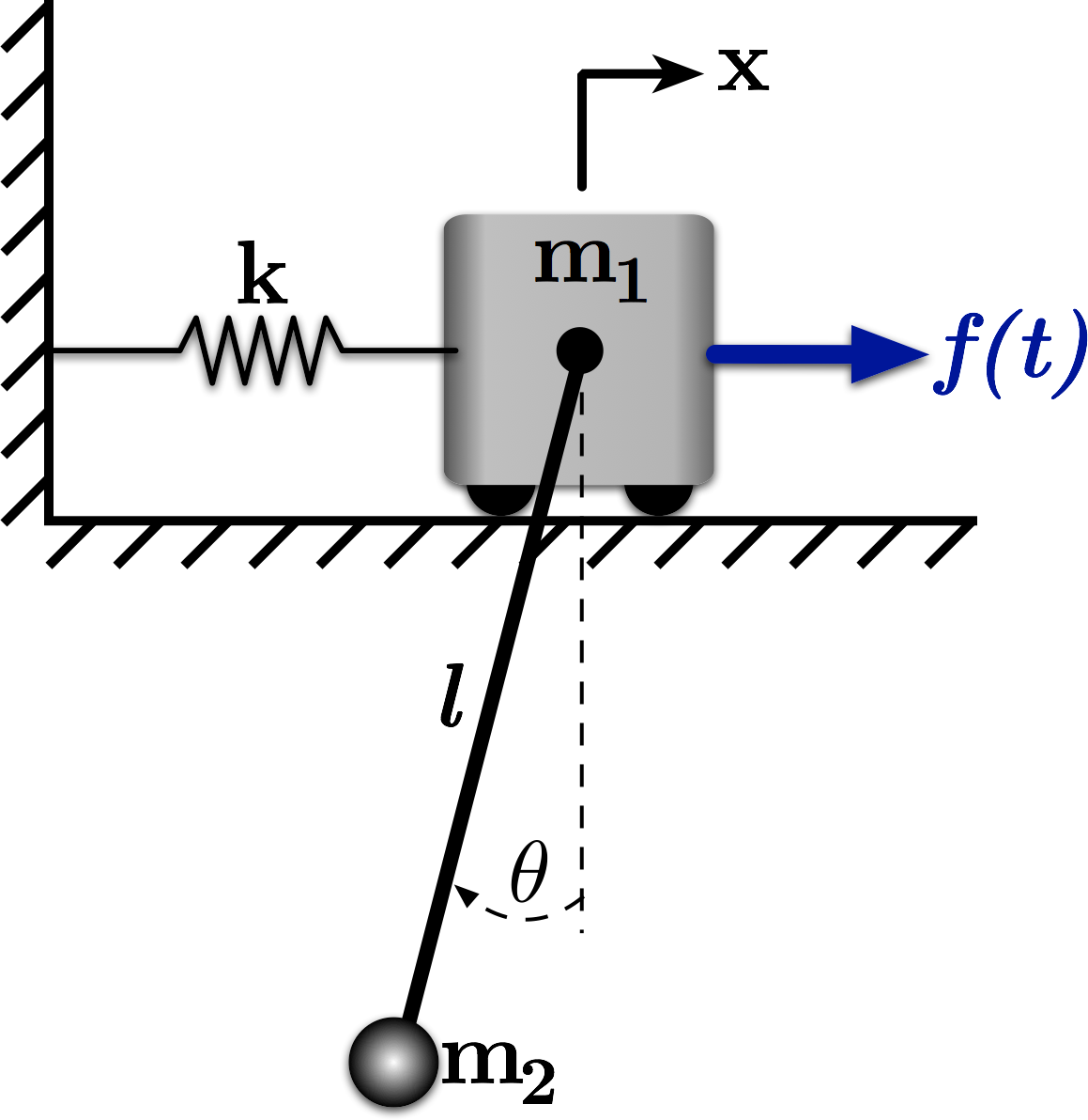
Figure 1: A Mass-Spring-Pendulum System
This notebook demonstrates the analysis of the system shown in Figure 1. Mass $m_1$ is attached to ground via a spring and constrained to move horizontally. Its horizontal motion from equilibrium is described by $x$. Mass $m_2$ is suspended from the center of $m_1$ via a massless, inextensible, inflexible cable of length $l$. The angle of this cable from horizontal is described by $\theta$. The linearized equations of motion for the system are:
$ \quad \left(m_1 + m_2\right) \ddot{x} - m_2 l \ddot{\theta} + k x = f $
$ \quad -m_2 l \ddot{x} + m_2 l^2 \ddot{\theta} + m_2 g l \theta = 0 $
We could also write this equation in matrix form:
$ \quad \begin{bmatrix}m_1 + m_2 & -m_2 l \\ -m_2 l & \hphantom{-}m_2 l^2\end{bmatrix}\begin{bmatrix}\ddot{x} \\ \ddot{\theta}\end{bmatrix} + \begin{bmatrix}k & 0 \\ 0 & m_2 g l\end{bmatrix}\begin{bmatrix}x \\ \theta\end{bmatrix} = \begin{bmatrix}f \\ 0\end{bmatrix}$
We'll use the Sympy tools to verify these equations of motion, then NumPy and SciPy to simulate the response of this system.
# Import the SymPy Module
import sympy

# Import the necessary sub-modules and methods for dynamics
from sympy.physics.mechanics import dynamicsymbols
from sympy.physics.mechanics import LagrangesMethod, Lagrangian
from sympy.physics.mechanics import Particle, Point, ReferenceFrame

# initiate better printing of SymPy results
sympy.init_printing()
# Define the genearlized coordinate
x, theta, f = dynamicsymbols('x theta f')

# Also define the first derivative
x_dot, theta_dot = dynamicsymbols('x theta', 1)

# Define the symbols for the other paramters
m1, m2, k, g, l, t = sympy.symbols('m_1, m_2, k, g, l, t')
# Define the Newtonian reference frame
N = ReferenceFrame('N')

# Define a body-fixed frame along the pendulum, with y aligned from m to the pin
A = N.orientnew('A', 'Axis', [-theta, N.z])

# Define the trolley point and its velocity
T = Point('T')
T.set_vel(N, x_dot * N.x)

# Treat the trolley as a particle
mtr = Particle('mtr', T, m1)

# Define the payload point and set its velocity
P = Point('P')
P.set_vel(N, x_dot * N.x - l * theta_dot * A.x)

# The payload is a particle (a point mass)
mp = Particle('mp', P, m2)

# Define the potential energy of the payload
mp.potential_energy = -m2 * g * l * sympy.cos(theta) # gravity
mtr.potential_energy = 1 / 2 * k * x**2              # spring potential

# Set up the force list - each item follows the form:
#    (the location where the force is applied, its magnitude and direction)
forces = [(T, f * N.x)]

# Form the Lagrangian, then simplify and print
L = Lagrangian(N, mtr, mp)
L.simplify()
# This creates a LagrangesMethod class instance that will allow us to form the equations of motion, etc
LM = LagrangesMethod(L, [x, theta], forcelist = forces, frame = N)
LM.form_lagranges_equations()
The LagrangesMethod class gives us lots of information about the system. For example, we can output the mass/inertia matrix and the forcing terms. Note that the forcing terms include what might be conservative forces and would therefore normally appear in a stiffness matrix.
# Output the inertia/mass matrix of the system
LM.mass_matrix
# Output the forcing terms of the system
LM.forcing
We can also use builtin functions to write the sytsem as a set of first order ODEs, suitable for simluation.
# Make the call to set up in state-space-ish form q_dot = f(q, t)
lrhs = LM.rhs()

# Simplify the results
lrhs.simplify()

# Output the result
lrhs
We can also linearize these equations with builtin SymPy methods. Let's do so about the $x = \dot{x} = \theta = \dot{\theta} = 0$ operating point. The resulting equations returned are a system of first order ODEs in state-space form:
$$ \dot{x} = Ax + Bu $$See the SymPy Documentation for much more information.
# Define the point to linearize around
operating_point = {x: 0.0, x_dot: 0.0, theta: 0.0, theta_dot: 0.0}

# Make the call to the linearizer
A, B, inp_vec = LM.linearize([x, theta], [x_dot, theta_dot],
                             op_point = operating_point,
                             A_and_B = True)
# simplify and print out the A matrix
A.simplify()
A
# simplify and print out the B matrix
B.simplify()
B
Checking the Result
These equations match the linearized equations of motion from the top of this notebook, if they are written as a system of first order ODEs, rather than two second-order ODEs. To begin, let's define a state vector $\mathbf{w} = \left[x \quad \theta \quad \dot{x} \quad \dot{\theta}\right]^T $
As mentioned above, we'll most often see the state space form writen as:
$ \quad \dot{x} = Ax + Bu $
where $x$ is the state vector, $A$ is the state transition matrix, $B$ is the input matrix, and $u$ is the input. We'll use $\mathbf{w}$ here and in the code to avoid confusion with our state $x$, the position of $m_1$.
To begin, let's write the two equations of motion as:
$ \quad \ddot{x} = \frac{1}{m_1 + m_2} \left(m_2 l \ddot{\theta} - k x + f \right)$
$ \quad \ddot{\theta}= \frac{1}{m_2 l^2} \left(m_2 l \ddot{x} - m_2 g l \theta\right) = \frac{1}{l}\ddot{x} - \frac{g}{l}\theta $
After some algebra and using the state vector defined above, we can write our equations of motion as:
$$ \dot{\mathbf{w}} = \begin{bmatrix}0 & 0 & 1 & 0\\ 0 & 0 & 0 & 1 \\ -\frac{k}{m_1} & -\frac{m_2}{m_1}g & 0 & 0 \\ -\frac{k}{m_1} & -\left(\frac{m_1 + m_2}{m_1}\right)\frac{g}{l} & 0 & 0 \end{bmatrix}\mathbf{w} + \begin{bmatrix}0 \\ 0 \\ \frac{1}{m_1} \\ \frac{1}{m_1 l} \end{bmatrix} f $$Now, we have the option of automating the creation of the functions necessary for use in the ODE solver, like we've done in some other notebooks. Here, let's manually generate the necessary functions to examine that case.
# import NumPy with namespace np
import numpy as np

# import the ode ODE solver
from scipy.integrate import odeint

# import the plotting functions from matplotlib
import matplotlib.pyplot as plt

# set up the notebook to display the plots inline
%matplotlib inline
# Define the system parameters
m1 = 10.0            # Trolley mass (kg)
m2 = 1.0             # Payload mass (kg)
g = 9.81             # Gravity (m/s^2)
k = 4 * np.pi**2     # Spring constant (N/m)
l = 2.0              # Cable length (m)
To use scipy.intergrate.odeint we need to define a funciton that represents the system of first order differential equations we want to solve. Here, that is simply the system of equations of motion. The odeint funciton requires the the arguments of this function be w, t, p, where w is the vector of states, t is the time, and p is a list of other parameters, as necessary. The function should returnn the system as a list.
We'll also define the forcing function, with arguments following the order of those requried by odeint.
# Define the system as a series of 1st order ODES (beginnings of state-space form)
def eq_of_motion(w, t, p):
    """
    Defines the differential equations for the coupled spring-mass system.

    Arguments:
        w :  vector of the state variables:
                  w = [x, theta, x_dot, theta_dot]
        t :  time
        p :  vector of the parameters:
                  p = [m1, m2, k, l, g, wf]

    Returns:
        sysODE : An list representing the system of equations of motion as 1st order ODEs
    """
    x, theta, x_dot,  theta_dot = w
    m1, m2, k, l, g, wf = p

    # Create sysODE = (x', theta', x_dot', theta_dot'):
    sysODE = [x_dot,
              theta_dot,
              -k/m1 * x - m2/m1 * g * theta + f(t,p)/m1,
              -k/(m1 * l) * x - (m1 + m2)/m1 * g/l * theta + f(t, p)/(m1 * l)]

    return sysODE


# Define the forcing function
def f(t, p):
    """
    Defines the forcing function

    Arguments:
        t : time
        p :  vector of the parameters:
             p = [m1, m2, k, l, g, wf]

    Returns:
        f : forcing function at current timestep
    """

    m1, m2, k, l, g, wf = p

    # Uncomment below for no force input - use for initial condition response
    #f = 0.0

    # Uncomment below for sinusoidal forcing input at frequency wf rad/s
    f = np.sin(wf * t)

    return f
# Set up simulation parameters

# ODE solver parameters
abserr = 1.0e-9
relerr = 1.0e-9
max_step = 0.01
stoptime = 25.0
numpoints = 2501

# Create the time samples for the output of the ODE solver
t = np.linspace(0.0, stoptime, numpoints)

# Initial conditions
x_init = 0.0                        # initial position
x_dot_init = 0.0                    # initial velocity
theta_init = 0.0                    # initial angle
theta_dot_init = 0.0                # initial angular velocity

wf = np.sqrt(k / m1)                # forcing function frequency

# Pack the parameters and initial conditions into arrays
p = [m1, m2, k, l, g, wf]
x0 = [x_init, theta_init, x_dot_init, theta_dot_init]
# Call the ODE solver.
resp = odeint(eq_of_motion, x0, t, args=(p,), atol=abserr, rtol=relerr,  hmax=max_step)
# Let's plot the trolly position and cable angle as subplots, to make it easier to compare

# Make the figure pretty, then plot the results
#   "pretty" parameters selected based on pdf output, not screen output
#   Many of these setting could also be made default by the .matplotlibrc file
fig, (ax1, ax2) = plt.subplots(1, 2, figsize=(12,4))

plt.subplots_adjust(bottom=0.12,left=0.17,top=0.96,right=0.96)
plt.setp(ax1.get_ymajorticklabels(),family='serif',fontsize=18)
plt.setp(ax1.get_xmajorticklabels(),family='serif',fontsize=18)
plt.setp(ax2.get_ymajorticklabels(),family='serif',fontsize=18)
plt.setp(ax2.get_xmajorticklabels(),family='serif',fontsize=18)

ax1.spines['right'].set_color('none')
ax1.spines['top'].set_color('none')
ax1.xaxis.set_ticks_position('bottom')
ax1.yaxis.set_ticks_position('left')
ax1.grid(True,linestyle=':',color='0.75')
ax1.set_axisbelow(True)

ax2.spines['right'].set_color('none')
ax2.spines['top'].set_color('none')
ax2.xaxis.set_ticks_position('bottom')
ax2.yaxis.set_ticks_position('left')
ax2.grid(True,linestyle=':',color='0.75')
ax2.set_axisbelow(True)


# Trolley Position plot
ax1.set_xlabel(r'Time (s)',family='serif',fontsize=22,weight='bold',labelpad=5)
ax1.set_ylabel(r'Displacement (m)',family='serif',fontsize=22,weight='bold',labelpad=10)
ax1.plot(t, resp[:,0], linewidth=2)


# Cable Angle plot
ax2.set_xlabel(r'Time (s)',family='serif',fontsize=22,weight='bold',labelpad=5)
ax2.set_ylabel(r'Angle (deg)', family='serif', fontsize=22, weight='bold',labelpad=10)
ax2.plot(t, resp[:,0] * 180/np.pi, linewidth=2)


# Adjust the page layout filling the page using the new tight_layout command
plt.tight_layout(pad=0.5)

# If you want to save the figure, uncomment the commands below.
# The figure will be saved in the same directory as your IPython notebook.
# Save the figure as a high-res pdf in the current folder
# savefig('MassSpringPend_Response.pdf', dpi=300)

fig.set_size_inches(18,6) # Resize the figure for better display in the notebook

Licenses
Code is licensed under a 3-clause BSD style license. See the licenses/LICENSE.md file.
Other content is provided under a Creative Commons Attribution-NonCommercial 4.0 International License, CC-BY-NC 4.0.
# This cell will just improve the styling of the notebook
from IPython.core.display import HTML
import urllib.request
response = urllib.request.urlopen("https://cl.ly/1B1y452Z1d35")
HTML(response.read().decode("utf-8"))