from IPython.core.display import HTML
css_file = 'stylesheets/custom.css'
HTML(open(css_file, "r").read())


Optimization and Machine
Learning with Python
This part of the advanced tutorial focuses more on some specific packages.
The topics covered in this part are:
- Optimization in Python with [Scipy](http://scipy.org/) and [APMonitor](http://apmonitor.com/wiki/index.php/Main/PythonApp).
- Easy and effective Machine Learning in Python with [Scikit-Learn](http://scikit-learn.org/stable/).
Presented on 2nd March, 2017 by Yiannis Hadjimichael and Uchenna Akujuobi.
Prerequisites: Basic and Intermediate tutorials or some experience with Python, Numpy, Scipy, Matplotlib (optional). Basic knowledge in machine learning and optimization.
1. Optimization in Python with Scipy and APMonitor
In this part, we'll learn how to solve optimization problems using the Scipy and Advanced Process Monitor (APMonitor) package for Python.
APMonitor Python is designed for large-scale optimization and accesses solvers of constrained, unconstrained, continuous, and discrete problems. It can solve a variety of problems in linear programming, quadratic programming, integer programming, nonlinear optimization, systems of dynamic nonlinear equations, and multiobjective optimization. It is free for academic and commercial use.
The current APMonitor Python version with examples can be found at http://apmonitor.com/wiki/index.php/Main/PythonApp.
For this tutorial we have already included the source python file (apm.py) in the git reposidory, as well as the .amp files for needed in the various examples.
APMonitor works both with Python and Matlab.
Optimization formulation
The general formulation of an optimization problem is to An optimization problem can be expressed in the following way:
- Given: a function $f : A \to R$ from some set $A$ to the set of real numbers
- Want to find a solution $x_0 \in A$ such that $f(x_0)$ is the minimum (or maximum) of $f(x)$ for all $x \in A$.
For example the standard form of a continuous optimization problem is:
$ \text{max (or min) } \mathbf{f(x)} $
$ \text{subject to } \\ $
$ \mathbf{lb} \le \mathbf{x} \le \mathbf{ub} \\ \mathbf{A x} \le \mathbf{b} \\ \mathbf{A}_\mathbf{eq} \mathbf{x} = \mathbf{b}_\mathbf{eq} \\ \mathbf{c_i(x) \ge 0} \quad \forall i=0,...,I \\ \mathbf{h_j(x) = 0} \quad \forall i=0,...,J \\ \mathbf{x \in R^n} $
where $\mathbf{f, c_i, h_j} :R^n \to R$.
According to the type of the objective function $\mathbf{f(x)}$ and constraints the optimization problem is either linear, quadratic, nonlinear, unconstrained, constrained etc.
How the APMonitor works
First, the package is called by
from apm import *
An online server and an application name must be then defined. e.g.
server = 'http://xps.apmonitor.com'
app = 'my_app'
The .apm file is then loaded which contains the setup of the problem in a similar fashion is defined mathematically.
Therefore the .apm file contains the objective function, optimization and control variables, fixed parameters and a set of
equations describing equality/inequality constraints or differential algebraic equations.
We load the setup file by
apm_load(s,a,'setup.apm')
Then depending on the nature of the optimization problem we can set variable options using the apm_option command.
Finally we solve the problem by
apm(server,app,'solve')
A detailed report is provided consisting of the optimization variables, equations used, and optimization solver, number of iterations, terminating conditions and tolerances, objective functions and optimizers and flags whether the optimiations was succesful or not.
The solution can be retrieved by
solution = apm_sol(server,app)
The best way to see how it works is to go through some examples.
Example 1 : Linear problem
A linear optimization problem has the following form:
$ \text{max (or min) } \mathbf{c}^T\mathbf{x} $
$ \text{subject to } \\ $
$ \mathbf{lb} \le \mathbf{x} \le \mathbf{ub} \\ \mathbf{A x} \le \mathbf{b} \\ \mathbf{A}_\mathbf{eq} \mathbf{x} = \mathbf{b}_\mathbf{eq} \\ \mathbf{x \in R^n} $
Consider the following problem:
$ \text{min} (15x_1 + 8x_2 + 80x_3) $
$ \text{subject to} $
$ x_1 + 2x_2 + 3x_3 <= 15 \\ 8x_1 + 15x_2 + 80x_3 <= 80 \\ 8x_1 + 80x_2 + 15x_3 <= 150 \\ -100x_1 - 10x_2 - x_3 <= -800 \\ 80x_1 + 8x_2 + 15x_3 = 750 \\ x_1 + 10x_2 + 100x_3 = 80 $
$\text{with } 4 <= x_1, -80 <= x_2 <= -8.$
The lp.apm file contains the descriprion of the model:
# %load scripts/session5/lp.apm
Model

  Variables
    x[1] = 4, >=4
    x[2] = -80, >=-80, <=-8
    x[3] = 0  >=-1e10, <=1e10
  End Variables

  Equations
    x[1] + 2*x[2] + 3*x[3] <= 15
    8*x[1] + 15*x[2] + 80*x[3] <= 80
    8*x[1] + 80*x[2] + 15*x[3] <= 150
   -100*x[1] - 10*x[2] - x[3] <= -800
    80*x[1] + 8*x[2] + 15*x[3] = 750
    x[1] + 10*x[2] + 100*x[3] = 80

    minimize  15*x[1] + 8*x[2] + 80*x[3]
  End Equations

End Model
We import the necessary packages and append to the path the location of apm.py in order to import the APM package.
%matplotlib inline
import numpy as np
import matplotlib.pyplot as plt
from random import randint
import sys
sys.path.append("scripts/session5/")
from apm import *
Then we choose the server and application name, load the model and option and solve it.
# server
server = 'http://xps.apmonitor.com'

# application + random number
app = 'lp' + str(randint(2,999))

# clear server
apm(server,app,'clear all')

# load model
apm_load(server,app,'scripts/session5/lp.apm')

# choose the solver
# 1=APOPT (active-set), 2=BPOPT (interior-point), 3=IPOPT (interior-point)
apm_option(server,app,'nlc.solver',1)

# solve
output = apm(server,app,'solve')
# retrieve solution
solution = apm_sol(server,app)
print(solution) # should print [ 9.89355041 -8. 1.5010645 ]
Solving the problem with scipy:
from scipy.optimize import linprog

# objective function
f = np.array([15, 8, 80])

# inequalities
A = np.array([[1, 2, 3], [8, 15, 80], [8, 80, 15], [-100, -10, -1]])
b = np.array([15, 80, 150, -800])

# equalities
Aeq = np.array([[80, 8, 15], [1, 10, 100]])
beq = np.array([750, 80])

# bounds
x0_bounds = (4, -80, None)
x1_bounds = (None, -8, None)

# solve
sol = linprog(f, A_ub=A, b_ub=b, A_eq=Aeq, b_eq=beq, bounds=list(zip(x0_bounds,x1_bounds)))

print('objFunValue: {:.16f}'.format(sol.fun)) # should print 204.48841578
print('x_opt: {}'.format(sol.x)) # should print [ 9.89355041 -8. 1.5010645 ]
We can easily verify that solution satisfies the constraints:
# error for equalitity constraints
print(np.linalg.norm(np.dot(Aeq,sol.x)- beq))

# inequalities
print(np.dot(A,sol.x)- b <= 0)
Example 2: Least square problem
Consider some 2D data. We would like to find a model to the measured data that minimizes the discrepancy between model predictions and the data. This can be formulated by minimizing the sum of the squares of the difference between values of model and measured data.
First create some data and plot them:
n = 200
x = np.linspace(0,2,n)
m = lambda x : 0.8*np.exp(-1.5*x)+1.2*np.exp(-0.8*x)
perturb = 0.5*np.random.uniform(0,1,n)
y = m(x)*(1.0+perturb)
plt.figure(figsize=(12,8), dpi=100) # changing figure's shape
plt.plot(x,y,'.')
plt.xlabel('x',fontsize=16) # horizontal axis name
plt.ylabel('y(x)',fontsize=16) # vertical axis name
plt.xticks(fontsize=14)
plt.yticks(fontsize=14)
plt.title('Sample data',fontsize=18) # title
plt.grid(True) # enabling grid
Now let's solve the least square problem:
"""
In this example we will search for z = (a, b, c, d)
that minimizes Sum_i || F(X_i;z) - Y_i ||^2
for the function
F(x) = a*exp(-b*x) + c*exp(-d*x)
"""
from scipy.optimize import least_squares

# function for computing residuals
def fun(z, x, y):
    return z[0]*np.exp(-z[1]*x) + z[2]*np.exp(-z[3]*x) - y

# initial estimate
x0 = np.array([0.2, 0.9, 1.9, 0.9])

sol_lsq = least_squares(fun, x0, args=(x, y))

# solution parameters
z = sol_lsq.x

residual = sum(sol_lsq.fun**2)

print('solution: '+str(z)+'\n||residuals||^2 = '+str(residual))
def fun(z, x, y):
    return z[0]*np.exp(-z[1]*x) + z[2]*np.exp(-z[3]*x)

plt.figure(figsize=(15,10), dpi=100)
plt.plot(x,y,'.')
plt.plot(x,fun(z,x,y),'r-',linewidth=1.5)
plt.xlabel('x',fontsize=16)
plt.ylabel('y',fontsize=16)
plt.title('Sample data',fontsize=18)
plt.grid(True) # enabling grid
Example 3: Nonlinear problem
Consider the following example of a non-linear problem (from http://apmonitor.com/wiki/index.php/Main/PythonApp)
# %load scripts/session5/nlp.apm
Model
  Variables
    x[1] = 1, >=1, <=5
    x[2] = 5, >=1, <=5
    x[3] = 5, >=1, <=5
    x[4] = 1, >=1, <=5
  End Variables

  Equations
    x[1] * x[2] * x[3] * x[4] > 25
    x[1]^2 + x[2]^2 + x[3]^2 + x[4]^2 = 40

    minimize  x[1] * x[4] * (x[1]+x[2]+x[3]) + x[3]
  End Equations
End Model
# server
s = 'http://xps.apmonitor.com'

# application + random number
a = 'app' + str(randint(2,999))

# clear server
apm(s,a,'clear all')

# load model
apm_load(s,a,'scripts/session5/nlp.apm')

# choose solver
# 1=APOPT (active-set), 2=BPOPT (interior-point), 3=IPOPT (interior-point)
apm_option(s,a,'nlc.solver',3)

# solve
output = apm(s,a,'solve')
print(output)
Get the solution
solution = apm_sol(s,a)
print(solution)
We can also see the results in the browser:
apm_web_var(s,a)
Now let's visualize the results
# create a mesh for x_2 and x_4
x = np.arange(1.0, 5.0, 0.1)
y = np.arange(1.0, 5.0, 0.1)
x2, x4 = np.meshgrid(x,y)

# since we can plot only against two variables we choose the optimal values for x_1 and x_3
x1 = solution['x[1]']
x3 = solution['x[3]']

# compute the objective function, the inequality and equality equation
obj = x1*x4*(x1+x2+x3) + x3
ic = x1*x2*x3*x4
eq = x1**2 + x2**2 + x3**2 + x4**2
Now let's make a contour plot
plt.figure(figsize=(10,10))
plt.title('NLP Contour Plot',fontsize=20)

CS = plt.contour(x2,x4,obj)
plt.clabel(CS,fontsize=14)
plt.xlabel(r'$x_2$',fontsize=18)
plt.ylabel(r'$x_4$',fontsize=18)
plt.xticks(fontsize=14)
plt.yticks(fontsize=14)

CS = plt.contour(x2,x4,ic,[25.,26.,27.,28.],colors='b',linewidts=[40.,3.,2.,1.])
plt.clabel(CS,inline=True,fontsize='x-large')
CS = plt.contour(x2,x4,eq,[40.],colors='r',linewidts=[4.])
plt.clabel(CS,inline=True,fontsize='x-large')
plt.show()
We can easily get the same solution using scipy:
from scipy.optimize import minimize

# objective function
def fun(x):
    return x[0] * x[3] * (x[0]+x[1]+x[2]) + x[2]
# or inline-function:
# fun = lambda x: x[0] * x[3] * (x[0]+x[1]+x[2]) + x[2]

# constraints
cons = ({'type':'ineq','fun':lambda x: x[0]*x[1]*x[2]*x[3]-25},{'type':'eq','fun':lambda x: x[0]**2+x[1]**2+x[2]**2+x[3]**2-40})

# bounds
x0_bounds = (1,1,1,1)
x1_bounds = (5,5,5,5)

# initial value
x0 = np.array([1,5,5,1])

# solve
sol = minimize(fun, x0, method='SLSQP', bounds=list(zip(x0_bounds,x1_bounds)), constraints=cons)

print('objFunValue: {:.16f}'.format(sol.fun))
print('x_opt: {}'.format(sol.x))
# solution with APMonitor
print(solution)
Example 4: Dynamic Programming
Consider now a reactor that converts a compound A to intermediate compound B and a final species C. The objective is to adjust the temperature (T) to maximize the concentration of compound B at the final time.
This example is taken from Dynamic Optimization Benchmarks.
The problem is described as follows:
$\text{max } x_2(t_f)$
subject to
$\dfrac{d x_1}{dt} = -k_1x_1^2 \\ \dfrac{d x_2}{dt} = k_1x_1^2 - k_2x_2$
with
$k_1 = 4000 \exp\left(\frac{-2500}{T}\right), \quad k_2 = 6.3\times 10^5 \exp\left(\frac{-5000}{T}\right),$
and
$x(0) = [1, 0], \quad 298 <= T <= 398, \quad t_f = 1.$
# %load scripts/session5/dae.apm
Model

  Parameters
    p
    t >=298 <=398
  End Parameters

  Variables
    x1 = 1
    x2 = 0
  End Variables

  Intermediates
    k1 = 4000 * exp(-2500/t)
    k2 = 6.2e5 * exp(-5000/t)
  End Intermediates

  Equations
    maximize p * x2

    $x1 = -k1 * x1^2
    $x2 = k1*x1^2 - k2*x2

    ! note: the $ denotes time differential
  End Equations

End Model
# %load scripts/session5/dae.csv
time,p
0,0
0.001,0
0.1,0
0.2,0
0.3,0
0.4,0
0.5,0
0.6,0
0.7,0
0.8,0
0.9,0
1.0,1
# specify server and application name
s = 'http://byu.apmonitor.com'
a = 'dynopt'

apm(s,a,'clear all')
apm_load(s,a,'scripts/session5/dae.apm')
csv_load(s,a,'scripts/session5/dae.csv')

apm_option(s,a,'nlc.nodes',4)
apm_option(s,a,'nlc.solver',1)
apm_option(s,a,'nlc.imode',6)
apm_option(s,a,'nlc.mv_type',1)

apm_info(s,a,'MV','t')
apm_option(s,a,'t.status',1)
apm_option(s,a,'t.dcost',0)

output = apm(s,a,'solve')
print(output)
y = apm_sol(s,a)

print('Optimal Solution: ' + str(y['x2'][-1]))
plt.figure(figsize=(12,12))

plt.subplot(211)
plt.plot(y['time'][1:],y['t'][1:],'r-s')
plt.legend('T',fontsize=18)
plt.ylabel('Manipulated',fontsize=18)
plt.xticks(fontsize=14)
plt.yticks(fontsize=14)

plt.subplot(212)
plt.plot(y['time'],y['x1'],'b-s')
plt.plot(y['time'],y['x2'],'g-o')
plt.legend(['x1','x2'],fontsize=18)
plt.ylabel('Variables',fontsize=18)
plt.xlabel('Time',fontsize=18)
plt.xticks(fontsize=16)
plt.yticks(fontsize=16)

plt.show()
Machine Learning in Python
Machine learning is a hot and popular topic nowadays. It is about building programs with tunable parameters that are adjusted automatically by adapting to previously seen data. It intervenes literally every sphere of our life ranging from science, engineering, and industry to economics, sociology, and even personal relationships. So if it is applicable everywhere, we need to have handy tools for doing machine learning.
# Start pylab inline mode, so figures will appear in the notebook
%pylab inline
1.1. Quick Overview of Scikit-Learn
Adapted from http://scikit-learn.org/stable/tutorial/basic/tutorial.html
# Load a dataset already available in scikit-learn
from sklearn import datasets
digits = datasets.load_digits()
type(digits)
digits.data
digits.target
from sklearn import svm
clf = svm.SVC(gamma=0.001, C=100.)
clf.fit(digits.data[:-1], digits.target[:-1])

print ("Original label:", digits.target[7])
print ("Predicted label:", clf.predict(digits.data[7].reshape(1,-1)))

plt.figure(figsize=(10, 10))
for i in range(10):
    plt.subplot(2, 5, i + 1)
    plt.imshow(digits.images[i], interpolation='nearest',vmax=16, cmap=plt.cm.binary)
1.2. Data representation in Scikit-learn
Adapted from https://github.com/jakevdp/sklearn_scipy2013
Data in scikit-learn, with very few exceptions, is assumed to be stored as a two-dimensional array, of size [n_samples, n_features], and most of machine learning algorithms implemented in scikit-learn expect data to be stored this way.
- n_samples: The number of samples: each sample is an item to process (e.g. classify). A sample can be a document, a picture, a sound, a video, an astronomical object, a row in database or CSV file, or whatever you can describe with a fixed set of quantitative traits.
- n_features: The number of features or distinct traits that can be used to describe each item in a quantitative manner. Features are generally real-valued, but may be boolean or discrete-valued in some cases.
The number of features must be fixed in advance. However it can be very high dimensional (e.g. millions of features) with most of them being zeros for a given sample. This is a case where scipy.sparse matrices can be useful, in that they are much more memory-efficient than numpy arrays.
1.2.1. Example: iris dataset
To understand these simple concepts better, let's work with an example: iris-dataset.
# Don't know what iris is? Run this code to generate some pictures.
from IPython.core.display import Image, display
display(Image(filename='figures/session5/iris_setosa.jpg'))
print ("Iris Setosa\n")

display(Image(filename='figures/session5/iris_versicolor.jpg'))
print ("Iris Versicolor\n")

display(Image(filename='figures/session5/iris_virginica.jpg'))
print ("Iris Virginica")
# Load the dataset from scikit-learn
from sklearn.datasets import load_iris
iris = load_iris()
type(iris) # The resulting dataset is a Bunch object
iris.keys()
print (iris.DESCR)
# Number of samples and features
iris.data.shape
print ("Number of samples:", iris.data.shape[0])
print ("Number of features:", iris.data.shape[1])
print (iris.data[0])
# Target (label) names
print (iris.target_names)
# Visualize the data
x_index = 0
y_index = 1

# this formatter will label the colorbar with the correct target names
formatter = plt.FuncFormatter(lambda i, *args: iris.target_names[int(i)])

plt.figure(figsize=(7, 5))
plt.scatter(iris.data[:, x_index], iris.data[:, y_index], c=iris.target)
plt.colorbar(ticks=[0, 1, 2], format=formatter)
plt.xlabel(iris.feature_names[x_index])
plt.ylabel(iris.feature_names[y_index])
Quick Exercise:
Change x_index and y_index and find the 2D projection of the data which maximally separate all three classes.
# your code goes here
1.2.2. Other available datasets
Scikit-learn makes available a host of datasets for testing learning algorithms. They come in three flavors:
- Packaged Data: these small datasets are packaged with the scikit-learn installation, and can be downloaded using the tools in
sklearn.datasets.load_* - Downloadable Data: these larger datasets are available for download, and scikit-learn includes tools which streamline this process. These tools can be found in
sklearn.datasets.fetch_* - Generated Data: there are several datasets which are generated from models based on a random seed. These are available in the
sklearn.datasets.make_*
visit http://scikit-learn.org/stable/datasets/ to learn more about the available Scikit-learn datasets
# Where the downloaded datasets via fetch_scripts are stored
from sklearn.datasets import get_data_home
get_data_home()
# How to fetch an external dataset
from sklearn import datasets
Now you can type datasets.fetch_<TAB> and a list of available datasets will pop up.
Exercise:
Fetch the dataset olivetti_faces. Visualize various 2D projections for the data. Find the best in terms of separability.
A sample preview of the faces can be found at http://www.cl.cam.ac.uk/research/dtg/attarchive/facesataglance.html
from sklearn.datasets import fetch_olivetti_faces
# your code goes here
# fetch the faces data
# Use a script like above to plot the faces image data.
# Hint: plt.cm.bone is a good colormap for this data.
1.3. Linear regression and classification
In this section, we explain how to use scikit-learn library for regression and classification. We discuss Estimator class - the base class for many of the scikit-learn models - and work through some examples.
from sklearn.datasets import load_boston
data = load_boston()
print (data.DESCR)
# Plot histogram for real estate prices
plt.hist(data.target)
plt.xlabel('price ($1000s)')
plt.ylabel('count')
Quick Exercise: Try sctter-plot several 2D projections of the data. What you can infer from the plots?
# Visualize the data
Every algorithm is exposed in scikit-learn via an Estimator object. For instance a linear regression is:
from sklearn.linear_model import LinearRegression
clf = LinearRegression()
clf.fit(data.data, data.target)
predicted = clf.predict(data.data)
# Plot the predicted price vs. true price
plt.scatter(data.target, predicted)
plt.plot([0, 50], [0, 50], '--k')
plt.axis('tight')
plt.xlabel('True price ($1000s)')
plt.ylabel('Predicted price ($1000s)')
Examples of regression type problems in machine learning:
- Sales: given consumer data, predict how much they will spend
- Advertising: given information about a user, predict the click-through rate for a web ad.
- Collaborative Filtering: given a collection of user-ratings for movies, predict preferences for other movies & users.
- Astronomy: given observations of galaxies, predict their mass or redshift
Another example of regularized linear regression on a synthetic data set.
import numpy as np
from sklearn.linear_model import LinearRegression

rng = np.random.RandomState(0)
x = 2 * rng.rand(100) - 1

f = lambda t: 1.2 * t ** 2 + .1 * t ** 3 - .4 * t ** 5 - .5 * t ** 9
y = f(x) + .4 * rng.normal(size=100)

plt.figure(figsize=(7, 5))
plt.scatter(x, y, s=4)
x_test = np.linspace(-1, 1, 100)  #generate numbers from -1 to 1

for k in [4, 9]:
    X = np.array([x**i for i in range(k)]).T
    X_test = np.array([x_test**i for i in range(k)]).T
    order4 = LinearRegression()
    order4.fit(X,y)
    plt.plot(x_test, order4.predict(X_test), label='%i-th order'%(k))

plt.legend(loc='best')
plt.axis('tight')
plt.title('Fitting a 4th and a 9th order polynomial')
# Let's look at the ground truth
plt.figure()
plt.scatter(x, y, s=4)
plt.plot(x_test, f(x_test), label="truth")
plt.axis('tight')
plt.title('Ground truth (9th order polynomial)')
Let's use Ridge regression (with l1-norm regularization)
from sklearn.linear_model import Ridge

for k in [20]:
    X = np.array([x**i for i in range(k)]).T
    X_test = np.array([x_test**i for i in range(k)]).T
    order4 = Ridge(alpha=0.3)
    order4.fit(X, y)
    plt.plot(x_test, order4.predict(X_test), label='%i-th order'%(k))
plt.plot(x_test, f(x_test), label="truth")
plt.scatter(x, y, s=4)
plt.legend(loc='best')
plt.axis('tight')
plt.title('Fitting a 4th and a 9th order polynomial')
plt.ylim?
Exercise:
For this exercise, you need to classify iris data with nearest neighbors classifier and with linear support vector classifier (LinearSVC).
In order to measure the performance, calculate the accuracy or just use clf.score function built-in into the Estimator object.
from __future__ import division  # turn off division truncation -- division will be floating point by default
from sklearn.neighbors import KNeighborsClassifier
from sklearn.svm import LinearSVC
from sklearn.datasets import load_iris
iris = load_iris()

# Splitting the data into train and test sets
indices = np.random.permutation(range(iris.data.shape[0]))
train_sz = int(floor(0.8*iris.data.shape[0]))
X, y = iris.data[indices[:train_sz],:], iris.target[indices[:train_sz]]
Xt, yt = iris.data[indices[train_sz:],:], iris.target[indices[train_sz:]]
# your code goes here
1.4. Approaches to validation and testing
It is usually an arduous and time consuming task to write cross-validation or other testing wrappers for your models. Scikit-learn allows you validate your models out-of-the-box. Let's have a look at how to do this.
from sklearn import model_selection
X, Xt, y, yt = model_selection.train_test_split(iris.data, iris.target, test_size=0.4, random_state=0)
print (X.shape, y.shape)
print (Xt.shape, yt.shape)
# Cross-validating your models in one line
svc = LinearSVC()
scores = model_selection.cross_val_score(svc, iris.data, iris.target, cv=5,)
print (scores)
print (scores.mean())
model_selection.cross_val_score?
# Calculate F1-measure (or any other score)
from sklearn import metrics
f1_scores = model_selection.cross_val_score(svc, iris.data, iris.target, cv=5, scoring='f1_macro')
print (f1_scores)
print (f1_scores.mean())
Quick Exercise: Do the same CV-evaluation of the KNN classifier. Find the best number of nearest neighbors.
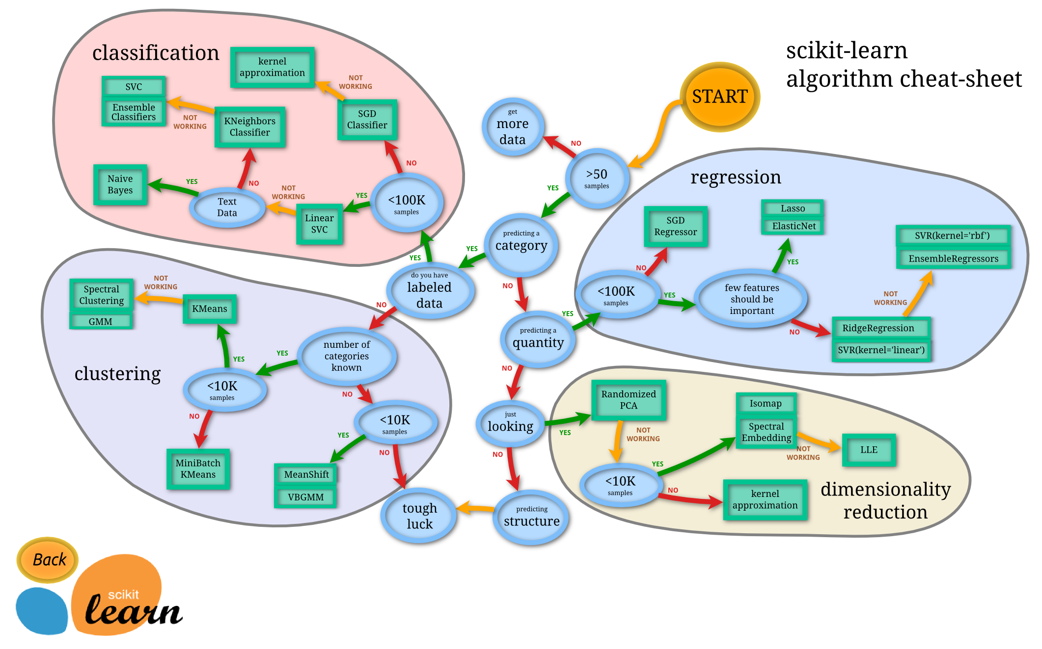
1.5. What to learn next?
If you would like to start using Scikit-learn for your machine learning tasks, the most right way is to jump into it and refer to the documentation from time to time. When you acquire enough skills in it, you can go and check out the following resources:
- A tutorial from PyCon 2013
- A tutorial from SciPy 2013 conference (check out the advanced track!)
Copyright 2017, ACM/SIAM Student Chapter of King Abdullah University of Science and Technology